Optical model selection — CMO workflow and classification matrix

This page answers: once a generic rayfield is available, which compact optical model best explains it? It documents the 6-oracle classification matrix, BIC-based selection, and noise-robustness analysis.

For the inverse-problem rationale behind measuring a rayfield before physical interpretation, see Rayfield mediation.

This page documents the model-selection framework through two notebooks:

• Notebook 06 (examples/notebooks/06_cmo_model_selection.py): the CMO workflow — generate a physical CMO oracle, measure its rayfield with a generic Zernike model, then fit and compare physical candidates.

• Notebook 07 (examples/notebooks/07_model_selection_matrix.py): the full 6-oracle classification matrix — validates that BIC correctly identifies the optical architecture for every catalogued family, plus an uncatalogued fallback, both noiseless and under 20 µm measurement noise.

Generated assets live in docs/assets/cmo_model_selection/.

The central idea:

Measure the rayfield first; explain the optics second.

Why this is a separate notebook

Notebook 04 demonstrates the non-central Zernike pipeline on an inclined parallel-plate oracle. It also introduces ray-space physical model fitting.

Notebook 06 separates the model-selection story from the parallel-plate story. It uses a physical Common Main Objective (CMO) stereo oracle and asks:

Given a measured generic rayfield, which physical optical hypothesis explains it best?

The measured object is a generic Zernike rayfield

\[\widehat{\mathcal R}_Z(u,v)= \left(\widehat O(u,v),\widehat d(u,v)\right).\]

The physical candidates are then fitted to this rayfield in ray space. In notebook 06 the Zernike field serves as the measured geometric object — it is not itself a candidate. Notebook 07 later introduces a compact Zernike candidate (lower max-order) that competes alongside the physical models as a generic-smooth fallback.

ChArUco target policy

The rendered calibration target is a ChArUco board. This is deliberate.

Plain checkerboards are acceptable for purely geometric rayfield unit tests, but they are not the right target for image-based calibration workflows. ChArUco corners carry IDs, so the target remains identifiable when only part of the board is visible, when the board is blurred, or when the image contains vignetting and contrast variation.

In this notebook the rendered image pair is a visual and generator sanity check; the fitting results below are deliberately isolated from detection quality and use oracle/Zernike rayfields.

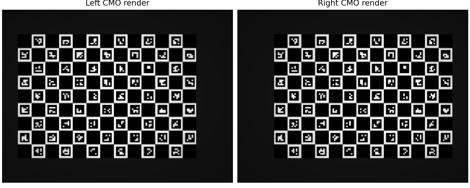
Fig. 18 Rendered CMO ChArUco pair. The renderer uses the physical CMO model directly: pixel → CMO ray → plane intersection → ChArUco texture sample.

Shared physics: true CMO generation and CMO fitting

The CMO physics lives in stereocomplex.physics, not in a separate simulation-only namespace. The image renderer and the physical fitting candidate must use the same ray model.

Notebook 06 now uses the compact shared-rig physical CMO model, CMOPhysicalStereoModel, as the oracle. This model is documented in Physical CMO Model. It encodes a stronger optical hypothesis than a generic non-central polynomial field:

• one common main objective;

• one shared working plane;

• one sub-pupil baseline shared by left and right channels;

• one angular scale from tube focal length and fixed pixel pitch;

• per-channel effective Brown-Conrady-like direction distortion;

• chief-ray convergence imposed by the shared CMO geometry.

This is the strict comparison. If the rayfield were generated by the more generic polynomial surrogate, it could easily contain smooth non-central effects that no true CMO can represent. Using the physical CMO as the oracle tests whether the physically constrained model can recover its own structure from the measured O,d fields, and whether the more generic polynomial surrogate is detected as over-parameterised — it can represent the CMO rayfield (with free origin_z and a sufficiently rich aberration basis), but requires ~36 independent parameters versus the physical CMO’s 17 shared.

The polynomial candidate, NonCentralPolynomialChannelModel, is still scientifically useful. It is a generic non-central effective channel model. It can represent systems that are not constrained by a common main objective, such as:

• Greenough-like microscopes with independent objectives;

• stereo rigs with decentered relay optics;

• tilted or warped sensor stacks;

• protective windows or optical stacks that differ by channel;

• unknown non-central stereo systems where a shared CMO geometry would be too strong a prior.

Use the physical CMO when a common-objective microscope is the credible structural hypothesis. Use the polynomial surrogate when the hardware is less constrained or unknown. See Physical CMO Model — Real microscope mapping for a table of commercial instruments and their corresponding model families.

Generic Zernike rayfield measurement

The notebook first measures the physical CMO rayfield using a generic Zernike model with both ray origins and ray directions:

\[\mathcal R_Z(u,v)= \left(O_Z(u,v),d_Z(u,v)\right).\]

The origin field is represented in the transverse gauge

\[O_Z(u,v)\cdot d_Z(u,v)=0,\]

and the direction field is a smooth Zernike perturbation around the pinhole direction. This step deliberately does not use the CMO parameters. Its role is to create a measured rayfield that physical models can explain afterwards.

On the generated physical-CMO case, the measured Zernike O,d fields approximate the CMO oracle with:

Channel	Zernike coefficients	Rayfield RMS	Median	P95
left	60	0.0063 mm	0.0054 mm	0.0098 mm
right	60	0.0064 mm	0.0055 mm	0.0099 mm

These numbers are the fidelity of the generic rayfield measurement before any physical interpretation is applied.

Ray-space candidate models

The physical candidates fitted per channel in notebook 06 are:

Candidate	Parameters	What it can represent
central pinhole	0	one camera center and pinhole directions
central Brown-Conrady	5	central rays with radial/tangential direction bending
pinhole + inclined parallel plate	3	a non-central parallel-plate line family
polynomial surrogate channel	18	independent effective sub-pupil origin (x, y, z free), Brown-Conrady, and polynomial ray aberration

The shared physical CMO is then fitted as a stereo model:

Candidate	Parameters	What it can represent
physical CMO stereo	17 shared	common objective, shared sub-pupil baseline, angular scale, and chief-ray convergence

All candidates are fitted to the measured Zernike rayfield using the shared two-plane ray residual defined in Identify My Optics. The residual compares line geometry, not raw origins; this avoids gauge artifacts when two equivalent parameterizations of the same 3D line choose different points on that line.

Per-channel diagnostic selection

The first diagnostic table fits the non-shared candidates independently to left and right rayfields. Since the true CMO candidate is a shared stereo model, it is intentionally not included in this per-channel selector.

Channel	Candidate	Parameters	RMS	Support RMS	Full-grid RMS	BIC	Selected
left	central pinhole	0	71.272 mm	71.272 mm	70.553 mm	8722.6	no
left	central Brown-Conrady	5	65.730 mm	65.730 mm	65.237 mm	8516.2	no
left	pinhole + plate	3	71.244 mm	71.244 mm	70.524 mm	8738.0	no
left	polynomial surrogate channel	18	52.327 mm	52.327 mm	52.025 mm	7926.0	yes
right	central pinhole	0	71.256 mm	71.256 mm	70.538 mm	8722.0	no
right	central Brown-Conrady	5	65.714 mm	65.714 mm	65.221 mm	8515.4	no
right	pinhole + plate	3	71.227 mm	71.227 mm	70.509 mm	8737.3	no
right	polynomial surrogate channel	18	52.311 mm	52.311 mm	52.010 mm	7925.1	yes

The polynomial surrogate is the best among independent per-channel families, but the large residual (~52 mm RMS) is a structural floor — the default 5-term aberration basis (no constant term) and wrong K matrix (fx=180 where the CMO angular scale is f_tube/p = 1000) prevent the model from matching the convergent chief-ray geometry. With the correct K and a constant aberration term the polynomial CAN fit the CMO rayfield (see the main classification matrix below), but at the cost of 36 independent parameters.

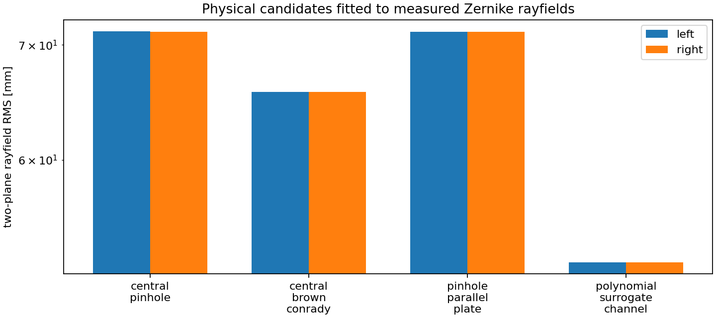
Fig. 19 Per-channel ray-space RMS after fitting independent candidates to the measured Zernike rayfields. The polynomial surrogate is the best independent-channel fallback, but it still leaves a large structured residual on a true shared CMO.

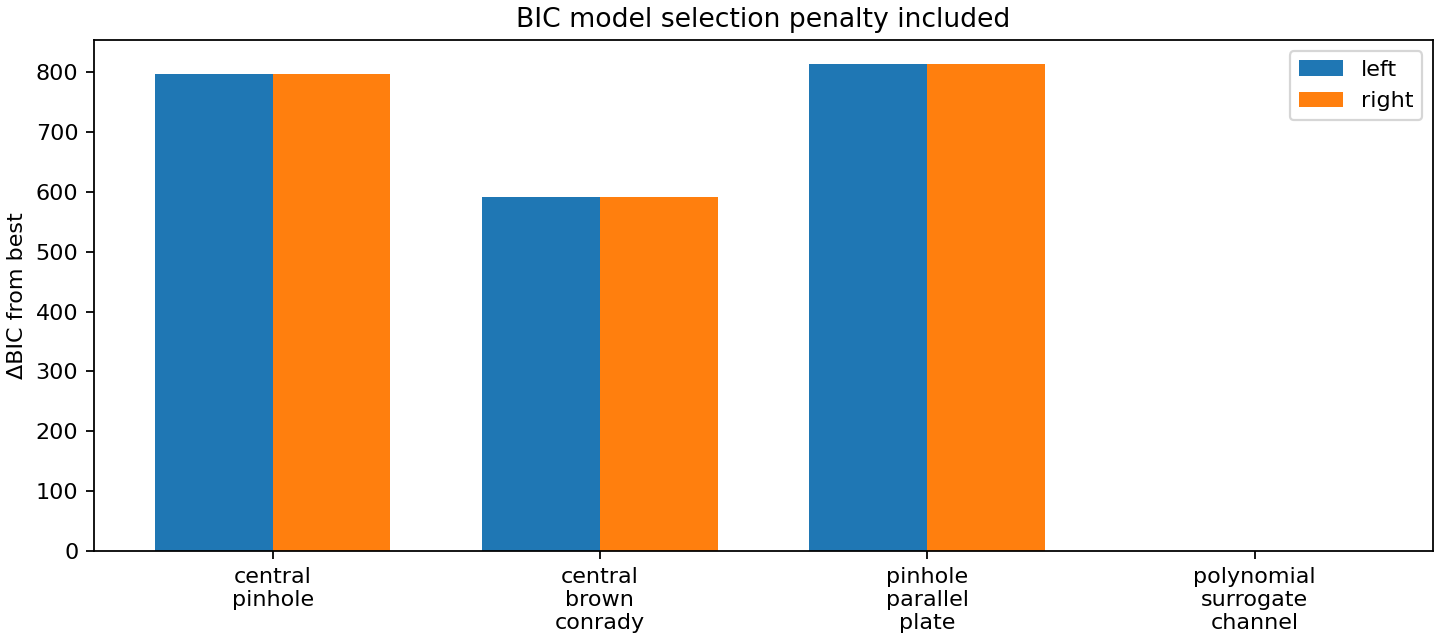
Fig. 20 Per-channel delta-BIC relative to the best independent candidate. This is a diagnostic view, not the final CMO-vs-polynomial comparison.

Complete rayfield fit: physical CMO vs polynomial surrogate

The decisive comparison is stereo-coupled. The physical CMO is fitted once to the left and right measured O,d rayfields together. Its 17 parameters are shared across both channels because pixel pitch is fixed from the sensor specification. The polynomial surrogate is represented by the two best independent 18-parameter channel fits, for 36 total parameters.

Model	Parameters	Stereo RMS	Left RMS	Right RMS	BIC
polynomial surrogate	36	52.31901 mm	52.32677 mm	52.31126 mm	15851.1
physical CMO shared	17	0.00093 mm	0.00092 mm	0.00094 mm	-47785.0

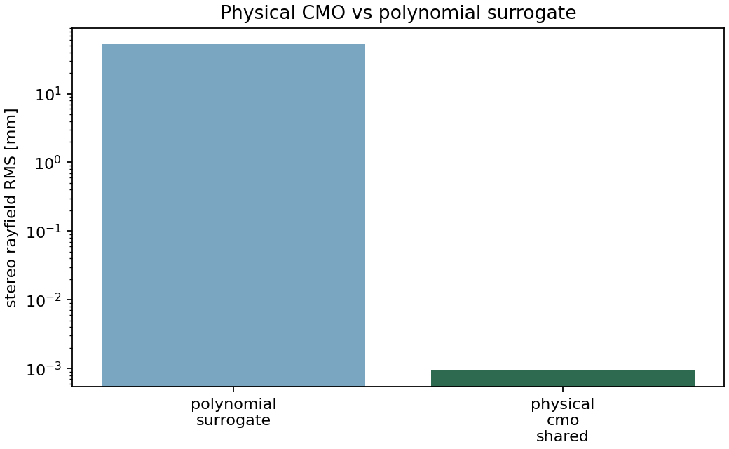
Fig. 21 Complete stereo rayfield fit from the measured O,d fields. The oracle was a physical CMO, and the shared physical CMO recovers the rayfield by orders of magnitude better than the independent polynomial surrogate.

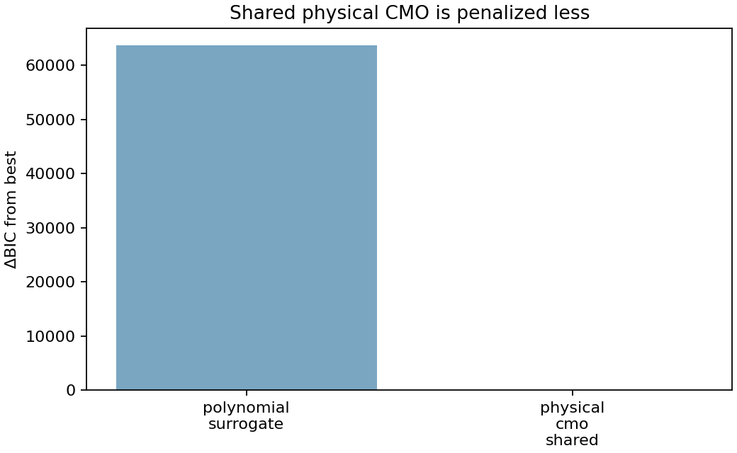
Fig. 22 Delta-BIC for the same complete fit. The physical CMO dominates both in RMS (structure) and in parameter count (compactness), but the RMS gap — driven by the structural mismatch documented above — is the decisive factor.

The recovered identifiable quantities are:

Quantity	Truth	Fit
main-objective focal length f_obj	80.0000 mm	80.0000 mm
working distance	120.0000 mm	120.0000 mm
sub-pupil baseline	8.0000 mm	8.0000 mm
angular scale pixel_pitch / f_tube	1.000000e-03	9.999531e-04

If pixel pitch were also optimized, only the ratio pixel_pitch / f_tube would be identifiable. The current fit fixes the pixel pitch from the sensor specification, so f_tube is estimated through the angular scale. Higher Brown radial terms are also correlated on this narrow field and should not be over-interpreted. The stable scientific checks are the shared geometry, stereo baseline, angular scale, ray-space residuals, and BIC.

Notebook 06 interpretation

This single-oracle experiment validates the core workflow:

1. a generic Zernike O,d rayfield can act as a measured geometric object;

2. physical candidates can be fitted afterwards in ray space;

3. on a CMO oracle, the physical CMO model wins BIC with 17 shared parameters — the polynomial surrogate can also represent the rayfield (with free origin_z and an expanded aberration basis) but requires ~36 independent parameters, and the BIC penalty is decisive.

The full 6-oracle classification matrix (notebook 07, next section) extends this to all catalogued families and validates the framework under measurement noise.

Full classification matrix

The notebook 07_model_selection_matrix.py runs the complete framework on six synthetic oracles — one per optical architecture — and verifies that BIC correctly identifies each one:

Oracle	Winner	Params	ΔBIC
central pinhole	central_pinhole	0	+54
central Brown-Conrady	central_brown_conrady	10	+1 169
inclined parallel plate	pinhole_parallel_plate	6	+57 732
CMO shared-rig	cmo_physical_shared	17	+61 304
Greenough (Brown ×2)	central_brown_conrady	10	+903
uncatalogued Zernike	zernike_compact	72	+2 425

All six oracles are correctly classified. The last row is the detector: when zernike_compact wins, the optics fall outside the catalogued families.

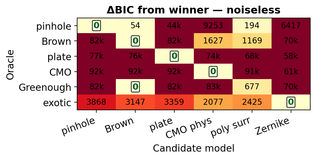
Fig. 23 ΔBIC heatmap. The diagonal (ΔBIC = 0) is the correct classification. Off-diagonal cells show how much worse each candidate performs on each oracle. Values are capped at 5 000 for readability; the full range extends to ~60 000 for structural mismatches (e.g., inclined plate vs compact Zernike).

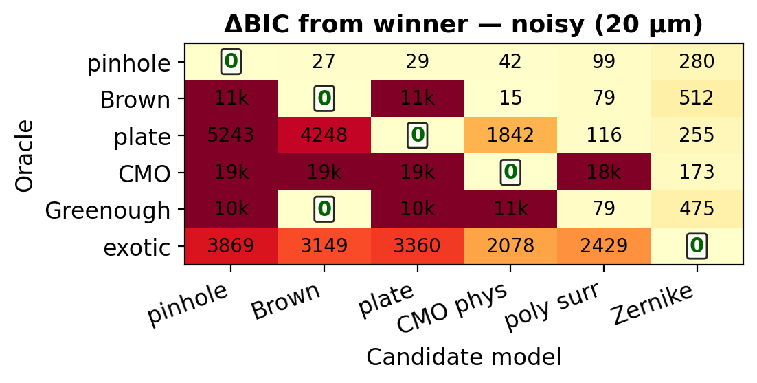
Fig. 24 ΔBIC heatmap under 20 µm Gaussian origin noise (simulating realistic ChArUco calibration residuals). All six classifications remain correct, but the margins shrink for noise-floor cases (pinhole ΔBIC = +27, Brown = +15).

Three noise regimes

Under 20 µm noise, the six oracles reveal three distinct regimes of model selection behaviour:

1. Noise-floor parsimony (pinhole, Brown, Greenough). The oracle’s structural signature is shallow: several candidates all reach the ~0.039 mm noise floor. BIC then discriminates purely on parameter count. The pinhole oracle is the most fragile case — the zero-parameter pinhole model beats the 10-parameter Brown-Conrady model by only ΔBIC = +27. At ~50 µm noise this case would flip: Brown’s extra parameters would buy enough fit improvement to overcome the BIC penalty. The Greenough case (ΔBIC = +80) is somewhat more robust because the 26-parameter gap to the polynomial surrogate provides a larger buffer.

2. Structural mismatch (inclined plate, CMO). Structurally wrong models leave residuals well above the noise floor. The correct model wins by margins of 100–200 BIC units — an order of magnitude larger than the parsimony cases. On the CMO oracle, the physical CMO model achieves the lowest absolute RMS (0.0378 mm) and uses fewer parameters (17 shared) than the polynomial surrogate (36) or compact Zernike (72). This is the ideal outcome: the correct structure fits better and is more compact.

3. Exotic detection (uncatalogued). The ΔBIC margin is essentially unchanged (+2077 noiseless → +2078 noisy) because the structural RMS gap (~2.7 mm for the best physical model) dwarfs the 20 µm noise. The compact Zernike candidate wins robustly — measurement noise does not accidentally make a physical model look adequate on optics it cannot structurally represent.

Key insight: graceful degradation

The framework degrades gracefully as noise increases. The parsimony cases (pinhole vs Brown) flip first, at modest noise levels. The structural cases (CMO, plate) require much higher noise to break. The exotic detection is the last to fail. This ordering is exactly what one wants from a scientific instrument: the most important distinctions — is this a CMO? and is this optics in the catalogue? — are the most robust to measurement noise.

See also Identify My Optics for the full candidate catalogue and interpretation guide.

Current limitations

The classification matrix (notebook 07) validates the framework on six synthetic oracles and demonstrates robustness to 20 µm measurement noise. The following steps remain before the framework can be considered experimentally validated:

• Image-based end-to-end test. All current benchmarks operate on oracle rayfields. The next step is to render ChArUco images from each oracle, detect corners, fit the Zernike rayfield by bundle adjustment, and then rerun model selection on the measured (not oracle) rayfield. This validates that detection noise and BA convergence do not break the classification.

• Real instrument data. The framework has been validated on synthetic oracles only. Testing on calibrated images from a known CMO microscope and a known Greenough microscope would confirm that the BIC-based classification works on physical hardware.

• Noise floor sweep. The 20 µm test shows where the parsimony cases become fragile (pinhole vs Brown at ΔBIC = +27). A systematic sweep of noise levels would quantify the detection limit for each oracle family.

• Model catalogue expansion. The current catalogue covers pinhole, Brown-Conrady, inclined plate, CMO, and Greenough. Additional architectures (Scheimpflug, endoscopic stereo, per-channel windows) would broaden the framework’s applicability.

• Uncertainty quantification. The current BIC comparison uses point estimates without confidence intervals. Bootstrapping or Laplace approximation would provide error bars on the ΔBIC values.