Inclined parallel-plate oracle and Zernike origin-field identification

This page documents the synthetic non-central stereo benchmark added for the experimental Zernike rayfield model.

The important point is the role separation:

• the inclined parallel plate is only an oracle used to generate physically plausible synthetic observations;

• the fitted model is not a plate model and never receives the plate parameters (eta, thickness, alpha, beta, d1);

• StereoComplex identifies a generic low-order Zernike rayfield. The staged baseline fits ray origins O(u,v) only; the complete geometric BA can also fit directions d(u,v), board poses, and the stereo rig.

Why the central model should fail here

A central pinhole camera assumes that every ray in a camera view starts from one fixed center:

\[X(\lambda)=C+\lambda d(u,v).\]

The parallel-plate oracle keeps the same outgoing direction as the pinhole ray, but shifts the physical ray laterally:

\[\mathcal R_{\mathrm{true}}(u,v)=\left(I_2(u,v), d_{\mathrm{pinhole}}(u,v)\right).\]

Therefore the data are intentionally non-central. If we reconstruct them with a central stereo model, the reconstruction is expected to be biased even in the noise-free case. That bias is the signal this benchmark is designed to detect.

The fitted model represents each ray with a canonical origin:

\[O(u,v)\cdot d(u,v)=0.\]

This does not mean that the oracle exit point I2 is set to zero. The generator keeps the physical I2; the fitted field uses a transverse gauge for identifiability. Oracle-vs-fit comparisons therefore use ray intersections with reference planes, not raw origin equality.

Theory: inclined parallel plate as an oracle

For a pixel (u,v) and pinhole intrinsics

\[\begin{split}K= \begin{pmatrix} f_x & 0 & c_x\\ 0 & f_y & c_y\\ 0 & 0 & 1 \end{pmatrix},\end{split}\]

the normalized pinhole direction is

\[x=\frac{u-c_x}{f_x},\qquad y=\frac{v-c_y}{f_y},\qquad s(u,v)= \frac{(x,y,1)^T}{\sqrt{x^2+y^2+1}}.\]

The inclined plate normal is parameterized by two tilts:

\[q(\alpha,\beta)= \frac{(\tan\alpha,\tan\beta,1)^T} {\sqrt{\tan^2\alpha+\tan^2\beta+1}}.\]

For the parallel-plate oracle, we compute the physical entry point I1, the direction inside the glass s_g, and the exit point I2:

\[c=q\cdot s,\qquad s_\perp=s-cq,\qquad \beta_g=\sqrt{1-\frac{\|s_\perp\|^2}{\eta^2}},\]

\[s_g=\frac{s_\perp}{\eta}+\beta_g q,\qquad I_1=\frac{d_1}{q\cdot s}s,\qquad I_2=I_1+\frac{e}{\beta_g}s_g.\]

The oracle ray is therefore

\[\mathcal R_\mathrm{oracle}(u,v)=\left(I_2(u,v),\,s(u,v)\right).\]

This is a useful synthetic generator because it creates a non-central ray family while keeping the direction field known and simple. The identification code does not fit e, eta, alpha, beta, or d1; those parameters are never passed to the Zernike fit.

Theory: canonical origin field

A 3D line is unchanged if its origin is moved along the line:

\[\left(O,d\right) \equiv \left(O+\lambda d,d\right).\]

The longitudinal component of O is therefore not identifiable from pure point-to-ray geometry. The fitted model fixes the gauge by representing the point on the ray closest to the camera origin:

\[O_c(u,v)=\left(I-dd^T\right)O_\mathrm{raw}(u,v), \qquad O_c(u,v)\cdot d(u,v)=0.\]

Why Zernike? A rayfield is a smooth vector-valued function on the sensor domain. Any low-order smooth basis — Legendre, Chebyshev, B-splines — could represent it compactly. Zernike polynomials are chosen not for an optical analogy (they were designed for wavefront phase, not for ray origins or directions) but for a structural reason: polar separability.

Zernike modes separate radial order :math:n from angular frequency :math:m. This matters because the dominant symmetries of a stereo system are angular, not Cartesian:

• :math:m=0 (rotationally symmetric modes) captures what is common to both optical channels — objective lens aberrations, field curvature.

• :math:m=1 (dipolar modes) captures left/right asymmetry — the signature of off-axis sub-pupils and per-arm misalignments.

• Higher :math:m captures quadrupole and finer angular structure.

On a Cartesian basis those same patterns would be spread across many coefficients — you could fit equally well, but you could not read the physics from the coefficient vector.

The sensor is rectangular and the pupil is circular; Zernike privileges the pupil geometry. The normalisation below maps the sensor rectangle onto the unit disk, accepting that the corners carry no information.

The Zernike field is defined on normalized image coordinates. With

\[\xi=2\frac{u}{W-1}-1,\qquad \zeta=2\frac{v}{H-1}-1,\qquad \rho=\frac{\sqrt{\xi^2+\zeta^2}}{\sqrt{2}},\]

the raw origin field is

\[O_\mathrm{raw}(u,v)= \sum_j \mathbf{o}_j Z_j(\rho,\theta), \qquad \mathbf{o}_j\in\mathbb R^3.\]

The staged origin-only ray model is

\[\mathcal R_\mathrm{fit}(u,v)= \left( \left(I-dd^T\right)O_\mathrm{raw}(u,v), d_\mathrm{pinhole}(u,v) \right).\]

Zero Zernike coefficients give O(u,v)=0, which is exactly the central pinhole baseline. That is the initialization and the baseline model, not the oracle.

Theory: direction field

The complete BA mode also identifies a smooth direction perturbation. It starts from the pinhole direction d0(u,v) and adds a transverse Zernike correction:

\[\delta d_\perp(u,v)= \left(I-d_0d_0^T\right) \sum_j \mathbf{a}_j Z_j(\rho,\theta),\]

\[d(u,v)= \operatorname{normalize}\left(d_0(u,v)+\delta d_\perp(u,v)\right).\]

The transverse projection removes the direction-scale gauge and keeps the parameterization well conditioned around a central initialization. In the parallel-plate oracle the true outgoing direction is still pinhole-like, so this block is mainly a stress test of the BA parameterization. In more general non-central optics it is the natural extension from an origin-field model to a generic pixel-to-line model.

Theory: fitting objective

For each observed board point, the known 3D point in the camera frame is P_k. The ray predicted by the current field is (O_k,d_k). The residual is the point-to-line vector:

\[r_k=\left(P_k-O_k\right)\times d_k.\]

The default implementation keeps board poses, stereo extrinsics, and directions fixed, and optimizes only the Zernike origin coefficients:

\[\min_\Theta \sum_k \rho\left(\|r_k\|\right) + \lambda \sum_j (1+n_j^2)\|\mathbf{o}_j\|^2.\]

This is intentional: the default benchmark isolates whether a compact O(u,v) field can explain non-central geometry.

The complete geometric bundle-adjustment mode is also available. It optimizes a smooth direction perturbation

\[d(u,v)=\operatorname{normalize} \left(d_0(u,v)+\delta d_\perp(u,v)\right),\]

where d0 is the pinhole direction and \delta d_\perp is a Zernike field projected transverse to d0. It can also optimize the board poses and the stereo transform T_{R\leftarrow L}. Both pose and rig updates use a compact SE(3) rotation-vector parameterization and weak regularization around the central initialization:

\[\min \sum_k \rho(\|r_k\|) + \lambda_O\|\Theta_O\|^2 + \lambda_d\|\Theta_d\|^2 + \lambda_\mathrm{pose}\|\Delta \xi_\mathrm{pose}\|^2 + \lambda_\mathrm{rig}\|\Delta \xi_\mathrm{rig}\|^2.\]

The regularization is not cosmetic: planar non-central calibration has gauge freedoms. Without weak priors, the optimizer can trade board motion, baseline, and rayfield deformation while preserving very small point-to-ray residuals.

Implementation details of the complete non-central BA

The implementation is in src/stereocomplex/calibration/fit_zernike_origin_field.py. This section states the exact optimization problem used by the benchmark, so the reported numbers can be audited from the code.

For a Zernike maximum order nmax, the code uses all real Zernike modes with radial order n <= nmax, including the constant and linear modes. Thus nmax=3 gives 10 modes and nmax=4 gives 15 modes. Each camera has its own origin coefficients, and, when direction fitting is enabled, its own direction coefficients:

\[\Theta_O^L,\Theta_O^R \in \mathbb R^{N_Z\times 3}, \qquad \Theta_d^L,\Theta_d^R \in \mathbb R^{N_Z\times 3}.\]

The complete optimized state is

\[x = \left[ \Theta_O^L,\Theta_O^R, \Theta_d^L,\Theta_d^R, \xi_{B,1},\ldots,\xi_{B,N_f}, \xi_{\mathrm{rig}} \right],\]

where the \Theta_d block is present only when optimize_directions=True, the board-pose increments are present only when optimize_board_poses=True, and the rig increment is present only when optimize_stereo_extrinsics=True. In the complete BA used for the rendered-image table, all three flags are enabled.

All pose parameters are represented by 6-vectors \xi=(\omega_x,\omega_y,\omega_z,t_x,t_y,t_z): the first three entries are a SciPy rotation vector and the last three entries are the translation in millimetres. The current implementation optimizes absolute SE(3) parameters but regularizes their difference from the initialization.

Frames and residuals

Board poses are represented first in the left-camera frame. For frame i and board point X_j^B, the left-camera point is

\[P_{ij}^L = T_{L\leftarrow B,i}\,X_j^B .\]

The stereo rig transform maps left-camera coordinates to right-camera coordinates:

\[P_{ij}^R = R_{R\leftarrow L}P_{ij}^L + t_{R\leftarrow L}.\]

For the observed left and right pixels (u_{ij}^L,v_{ij}^L) and (u_{ij}^R,v_{ij}^R), the fitted fields return

\[(O_{ij}^L,d_{ij}^L)=\mathcal R_L(u_{ij}^L,v_{ij}^L), \qquad (O_{ij}^R,d_{ij}^R)=\mathcal R_R(u_{ij}^R,v_{ij}^R).\]

The residuals are 3D point-to-line vectors:

\[r_{ij}^L = (P_{ij}^L-O_{ij}^L)\times d_{ij}^L, \qquad r_{ij}^R = (P_{ij}^R-O_{ij}^R)\times d_{ij}^R.\]

The directions are unit-normalized at every evaluation. The residual components therefore have units of millimetres. No pixel-noise covariance weighting is applied in the current implementation; all observed point-to-ray residual components are passed to SciPy in millimetres.

Objective and robust loss

The vector passed to SciPy is the concatenation of all residual components and all active regularization pseudo-residuals. With all blocks active, the objective can be read as

\[\min_x \rho_{\mathrm{data}}(x) + R_O(x) + R_d(x) + R_{\mathrm{pose}}(x) + R_{\mathrm{rig}}(x).\]

The terms are

\[\rho_{\mathrm{data}}(x)= \sum_{i,j}\rho(r_{ij}^L)+\rho(r_{ij}^R),\]

\[R_O = \lambda_O\left( \|\sqrt{w}\Theta_O^L\|^2+ \|\sqrt{w}\Theta_O^R\|^2 \right),\]

\[R_d = \lambda_d\left( \|\sqrt{w}\Theta_d^L\|^2+ \|\sqrt{w}\Theta_d^R\|^2 \right),\]

\[R_{\mathrm{pose}} = \lambda_{\mathrm{pose}}\|\xi_B-\xi_{B,0}\|^2, \qquad R_{\mathrm{rig}} = \lambda_{\mathrm{rig}}\|\xi_{\mathrm{rig}}-\xi_{\mathrm{rig},0}\|^2 .\]

Here \rho is the robust loss chosen in scipy.optimize.least_squares. The benchmarks use loss="huber", method="trf" and f_scale=1.0, so the Huber transition is at roughly one millimetre per residual component. The Zernike regularization weights increase with radial order:

\[w_j = 1+n_j^2 .\]

In the actual residual vector, regularization is appended as \sqrt{\lambda}\sqrt{w_j}\theta_j, which is why the table below lists the \lambda values, not their square roots.

Initialization and benchmark parameters

The BA starts from the central initialization:

• O(u,v)=0 for both cameras;

• \delta d(u,v)=0, so directions initially equal the pinhole directions;

• board poses are the initial left-camera board poses provided to the function;

• the rig is initialized from T_right_left_initial.

In the synthetic benchmark these initial board poses and rig are the known central/oracle geometry, so the rendered-image experiment should be read as a front-end and non-central BA wiring test, not yet as a fully blind real-camera calibration. The rendered images then replace the oracle pixels by OpenCV (or Ray2D-refined) detections before the same BA is run.

The numerical settings used by the documented benchmarks are:

Case	nmax	lambda_O	lambda_d	lambda_pose	lambda_rig	max_nfev
O-only geometric benchmark	4	1e-3	inactive	inactive	inactive	200
Full geometric BA	3	1e-5	1e-2	10	100	100
Rendered-image BA	3	1e-5	1e-2	100	1000	200

These relatively strong pose and rig priors in the rendered-image BA are intentional. With a planar target and a non-central rayfield, the problem has practical gauge freedoms: without priors, pose, baseline and rayfield deformation can compensate one another while keeping small point-to-ray residuals.

From geometric observations to image-based identification

The present page validates two levels. First, it validates the geometric core from image coordinates associated with planar board points. Second, it renders actual ChArUco images from the non-central oracle, adds vignetting, spatially varying blur, and sensor noise, detects the board with OpenCV, and feeds those detected 2D observations into the same complete BA. The default O-only fit still uses known poses and rig to isolate expressivity. The complete BA fit starts from the same central initialization but optimizes O(u,v), d(u,v), board poses, and the stereo rig.

The image-based path is staged deliberately so that failures can be diagnosed:

Stage	Input observations	Unknowns optimized	Purpose
0. Geometric oracle (default)	synthetic 2D points	O(u,v) only	isolate non-central identifiability
1. Image detection	rendered ChArUco images	O(u,v) only	measure detector/rasterization bias
2. Full geometric BA (implemented here)	synthetic image coordinates	O(u,v) + d(u,v) + board poses + rig	test the full non-central parameterization
3. Detected-image BA (implemented here)	rendered/detected images	same unknowns as stage 2	test recovery from OpenCV detector outputs
4. Real-image BA	real stereo images	same unknowns as stage 2	validate deployment outside the synthetic oracle

The practical question behind stages 2–3 is:

starting from a central initialization and unknown calibration poses/rig, can the optimizer recover the same reconstruction quality as the staged geometric identification benchmark?

That BA version now exists at both the geometric-observation level and the rendered-image level: it optimizes O(u,v), d(u,v), board poses, and the stereo rig from OpenCV ChArUco detections. The central initialization is not a competitor in that experiment; it is the starting point used to make the nonlinear problem well posed.

Two diagnostics remain mandatory before treating this as a mature calibration workflow:

• train/test pose split: reconstruction and ray-gap metrics must be reported on held-out board poses, not only on the fitted poses;

• support-aware rayfield error: rayfield errors should be separated between the observed calibration support and the full image, because corner errors are often extrapolation errors rather than in-support identification errors.

The current implementation therefore answers three questions: “is the O(u,v) model expressive enough when the geometry is known?”, “does the full non-central BA over (O,d,poses,rig) have the right optimization wiring on image coordinates?”, and “does the same BA remain useful when those image coordinates come from an OpenCV detector on rendered images?” The next experiment must answer whether the same behaviour holds on real images and held-out poses.

Theory: reconstruction comparison

The central baseline uses

\[O_L=0,\qquad O_R=C_R,\]

with pinhole directions. The identified model uses

\[(O_L(u_L,v_L),d_L(u_L,v_L)),\qquad (O_R(u_R,v_R),d_R(u_R,v_R)).\]

Both are triangulated by closest approach of two 3D rays. If the central model is forced onto non-central oracle data, its rays are geometrically biased. If the identified O(u,v) field is correct, the two stereo rays become consistent and their midpoint recovers the board point.

Reproduce

This page is generated by the example script docs/examples/parallel_plate_origin_field_demo.py. The script intentionally uses the same public experimental API as the notebook.

Generate the figures and summary table:

.venv/bin/python docs/examples/parallel_plate_origin_field_demo.py

For a guided, editable walkthrough, open the notebook:

jupyter lab examples/notebooks/04_parallel_plate_origin_field.ipynb

The companion plain-Python export is:

examples/notebooks/04_parallel_plate_origin_field.py

The notebook follows this page: it first motivates why central stereo is wrong for this oracle, then runs the public experimental API, then displays the same error figures used below.

Run the complete local validation:

PYTHON=.venv/bin/python bash scripts/validate_local.sh

Reconstruction results

The benchmark uses a synthetic stereo rig with two inclined plates and a board observed at several depths. Two cases are shown:

• noise-free oracle: only model mismatch is present;

• 0.05 px observation noise: a small image-space perturbation is added.

We report an additional oracle reference: reconstruction with the exact parallel-plate rayfield evaluated at the observed pixels. In the noisy case this is not a strict lower bound for a global estimator, because a smooth fitted field can denoise observations using the known 3D board geometry. It is however the right scale for the raw-pixel noise floor.

Case	Model	RMS (mm)	Med. (mm)	P95 (mm)	Gap RMS (mm)
Noise-free	Central stereo	2.169	2.168	2.694	0.126
Noise-free	Oracle clean	~0	~0	~0	~0
Noise-free	Fitted O(u,v)	0.00994	0.00501	0.0213	0.000484
Noise-free	BA O+d+poses+rig	0.0153	0.00975	0.0310	0.0000565
0.05 px noise	Central stereo	2.310	2.257	3.040	0.154
0.05 px noise	Oracle noisy	0.801	0.538	1.644	0.0856
0.05 px noise	Fitted O(u,v)	0.784	0.521	1.556	0.0849
0.05 px noise	BA O+d+poses+rig	0.760	0.506	1.436	0.0831

The improvement factors are:

Case	RMS factor	Median factor	P95 factor
Noise-free	218.2x	432.4x	126.6x
0.05 px noise	2.94x	4.33x	1.95x

These numbers are the expected behaviour. In the noise-free case, the central model is wrong by construction, so the identified origin field removes almost all of the non-central bias. The experimental BA mode, which additionally fits d(u,v), the board poses, and the stereo rig, reaches the same scale without being limited to an O-only model (0.015 mm RMS in the noise-free case). With pixel noise, both the O-only fit and the BA fit reach the same scale as the oracle evaluated at noisy pixels (0.784 mm and 0.760 mm vs 0.801 mm RMS). The limiting factor is therefore the observation noise, not a failure of the non-central model.

A back-of-the-envelope stereo propagation gives the same order of magnitude:

\[\sigma_Z \approx \frac{Z^2}{fB}\sqrt{2}\,\sigma_\mathrm{px} \approx \frac{800^2}{620\times 90}\sqrt{2}\times 0.05 \approx 0.8~\mathrm{mm}.\]

This is why the noisy result should be interpreted as near the expected stereo-noise floor for this geometry.

From measured rayfield to physical model: fitting a thin parallel plate

The previous sections fit a generic Zernike rayfield. We can now use that rayfield as a measured geometric object and ask a different question:

can a low-dimensional physical model explain the measured non-central rayfield?

This is not the same as fitting the glass plate directly from ChArUco pixels. The physical model is fitted after the generic rayfield has been identified. This turns the optical inverse problem into a model-selection problem in the space of 3D rays:

\[\theta^\star = \arg\min_\theta D^2 \left( \widehat{\mathcal R}_Z, \mathcal R_{\mathrm{plate}}(\theta) \right).\]

Here \widehat{\mathcal R}_Z is the measured Zernike rayfield and \mathcal R_{\mathrm{plate}}(\theta) is a pinhole + inclined parallel-plate rayfield. In this first implementation, the fitted physical parameters are \theta=(\alpha,\beta,e) for each camera, with \eta=1.5 fixed. The plate distance d1 is not fitted because changing it moves I2 along the emergent ray and therefore does not change the 3D line.

The rayfield distance is computed by intersections with two reference planes:

\[D^2 = \sum_k \left|A_Z^k-A_{\mathrm{plate}}^k\right|^2 + \left|B_Z^k-B_{\mathrm{plate}}^k\right|^2, \qquad A=\mathcal R\cap\Pi_{z_0},\quad B=\mathcal R\cap\Pi_{z_1}.\]

Raw origins are never compared directly: the oracle keeps the physical exit point I2, while the measured Zernike field uses a transverse gauge. The physical fit is therefore an interpretation of the measured rayfield, not a replacement for the generic identification step.

For this physical-compression step we use a wider-coverage synthetic variant: the calibration board is larger and the poses are deliberately shifted toward the image borders. This is important because the fitted physical model is judged as a rayfield, not only by 3D reconstruction on a few board poses. The cyan points in the heatmap below show the actual observed support.

On that noise-free wide-coverage benchmark, fitting independent physical plates to the measured left and right Zernike fields gives:

Camera	alpha (deg)	beta (deg)	e (mm)	Support RMS	Full-grid RMS
Left	13.000	5.000	16.000	0.00020 mm	0.0016 mm
Right	10.002	7.001	13.998	0.00031 mm	0.0051 mm

For comparison, the true oracle parameters are (13 deg, 5 deg, 16 mm) on the left and (10 deg, 7 deg, 14 mm) on the right. With the edge-coverage poses extending observations to all image borders, the fitted parameters recover the oracle to within a thousandth of a degree and a thousandth of a millimetre. The full-grid residual remains slightly larger than the support residual: the Zernike field is measured from finite calibration poses, while the physical plate extrapolates globally from only three parameters.

The reconstruction comparison is:

Model	RMS 3D	Median 3D	P95 3D	Ray gap RMS
Central	2.731 mm	—	—	—
Zernike initial	0.00107 mm	—	—	—
Pinhole + fitted plate	0.000602 mm	0.000381 mm	0.00125 mm	0.0000576 mm
Oracle	~0	~0	~0	~0

The same physical interpretation was also run with 0.05 px observation noise on the wide-coverage synthetic dataset:

Model	RMS 3D
Central	2.796 mm
Zernike initial	0.676 mm
Pinhole + fitted plate	0.679 mm
Oracle at observed pixels	0.682 mm

The fitted physical plate is therefore no longer limited by the non-central model: it sits at the same scale as the oracle evaluated at noisy pixels. In this regime, the residual error is dominated by image-coordinate noise rather than by the compact physical model.

With adequate image coverage, the three-parameter physical model slightly outperforms the generic Zernike rayfield on 3D reconstruction (0.000602 mm vs 0.00107 mm RMS). This is expected: once the Zernike field is measured over the full image, the physical model can compress it to near-perfect accuracy over all pixels, not just the observed support. The value of the fitted plate is therefore compression, generalization, and interpretability: it explains the entire non-central rayfield with six scalar parameters for the stereo pair (alpha, beta, e per camera, with eta fixed), instead of a larger Zernike coefficient field.

The stability of the physical interpretation was checked by refitting the plate on 16 random subsets of the observed support. On this noise-free benchmark, the bootstrap standard deviations are small:

Camera	alpha mean +/- std	beta mean +/- std	e mean +/- std
Left	13.0002 +/- 0.0001 deg	5.0001 +/- <0.0001 deg	16.0000 +/- 0.0001 mm
Right	10.0008 +/- 0.0001 deg	7.0003 +/- 0.0001 deg	13.9994 +/- 0.0001 mm

This is not meant as a full uncertainty budget; it is a quick conditioning check. It shows that, once the Zernike rayfield has been measured with broad image support, the physical compression step is numerically stable.

Finally, the ray-space fit is now exposed as a generic optical model-selection diagnostic. The Zernike rayfield is the measured object; the physical candidates are judged by how well they compress and explain it. The mathematical definitions of the central pinhole, central Brown-Conrady, inclined parallel-plate, CMO channel, two-plane residual, AIC and BIC are centralized in Identify My Optics. This page keeps only the inclined-plate benchmark results.

The table below reports the average left/right RMS distance to the measured Zernike rayfield:

Candidate model	Observed support RMS	Full-grid RMS	Interpretation
Central pinhole	2.990 mm	3.714 mm	wrong central model
Central Brown-Conrady	2.143 mm	2.649 mm	bends directions, but cannot create O(u,v)
Pinhole + inclined plate	0.000258 mm	0.00335 mm	best compact physical explanation

The corresponding stereo-pair BIC values are +1052 for the central pinhole, -10772 for Brown-Conrady, and -306399 for the inclined plate. Lower is better, so both RMS and BIC select the inclined-plate model. This does not mean that StereoComplex fit the plate directly from pixels. It means that the measured rayfield contains enough information to reject central alternatives in ray space. The Brown-Conrady row is a misspecification test: as defined in Identify My Optics, it is central and therefore cannot reproduce the pixel-dependent origin field of the plate oracle.

The reconstruction comparison for the physical candidates is:

Model	RMS 3D	Ray gap RMS
Central pinhole	2.731 mm	—
Central Brown-Conrady fit to rayfield	3.888 mm	0.204 mm
Zernike initial	0.00107 mm	—
Pinhole + fitted plate	0.000602 mm	0.0000576 mm
Oracle	~0	~0

Brown-Conrady is not selected, and its stereo reconstruction is worse here because each camera bends directions independently while remaining central. The ray-space score is the primary diagnostic; the reconstruction table shows the same qualitative failure mode.

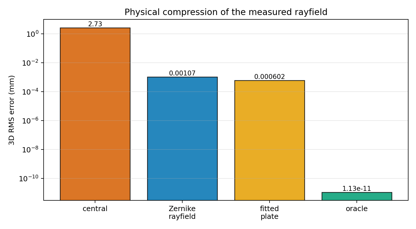
Fig. 25 Physical compression of the measured rayfield. With full-image edge coverage, the three-parameter plate model achieves slightly better 3D reconstruction than the generic Zernike field (0.00060 mm vs 0.00107 mm RMS), because it generalizes over the entire pixel domain rather than interpolating within the observed support.

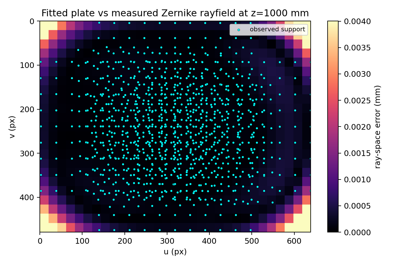
Fig. 26 Ray-space residual between the fitted plate model and the measured Zernike rayfield on the z=1000 mm plane. Cyan points show the observed calibration support. Errors outside that support mostly measure extrapolation differences.

Fig. 27 Bootstrap stability of the physical interpretation. The fitted parameters stay close to the oracle values when the plate is refitted on random subsets of the observed support.

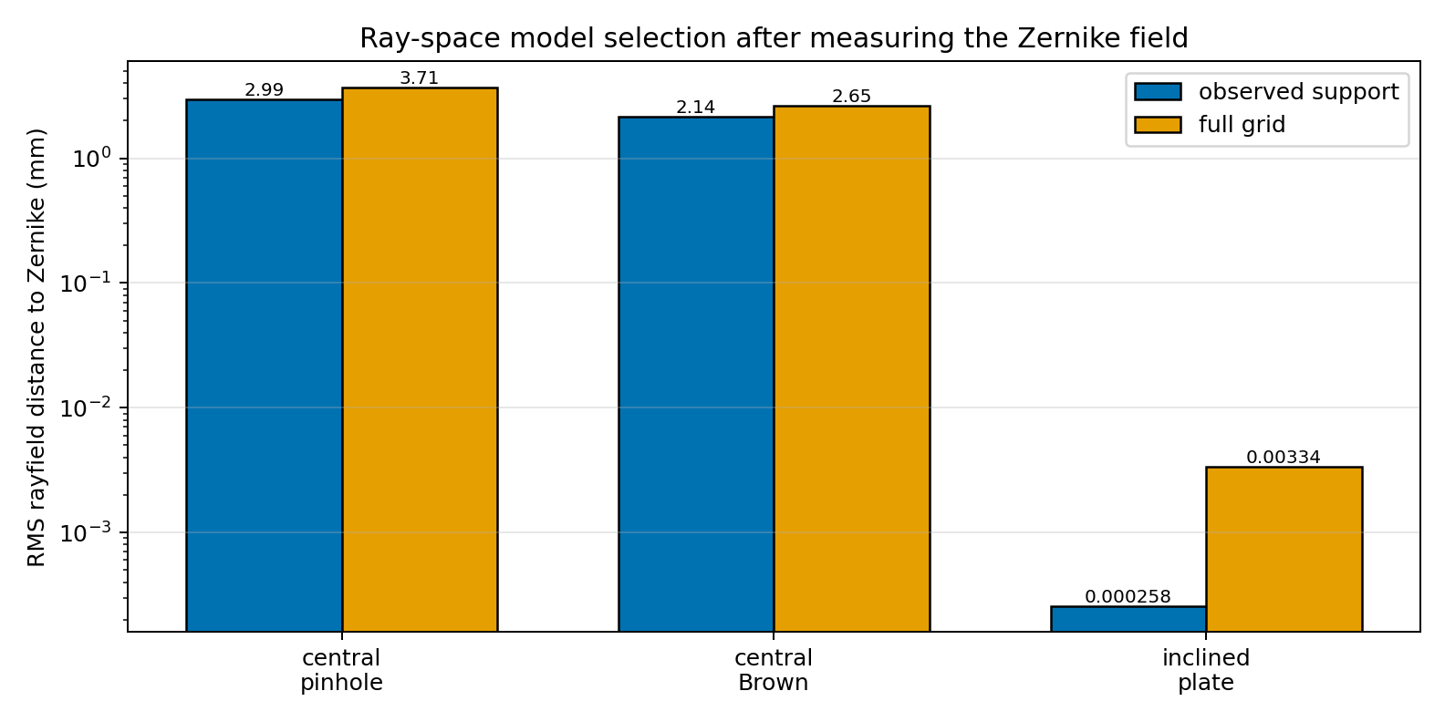
Fig. 28 Ray-space model selection after the generic Zernike rayfield has been measured. The inclined parallel-plate model is the only compact candidate that explains the measured non-central field at both support points and across the image grid.

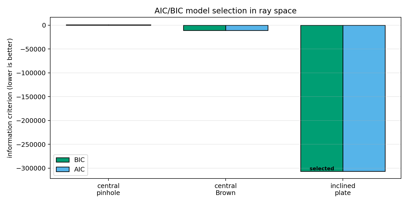
Fig. 29 Information-criterion view of the same model-selection problem. The plate wins despite using more parameters than the pinhole model because its ray-space residual is orders of magnitude lower.

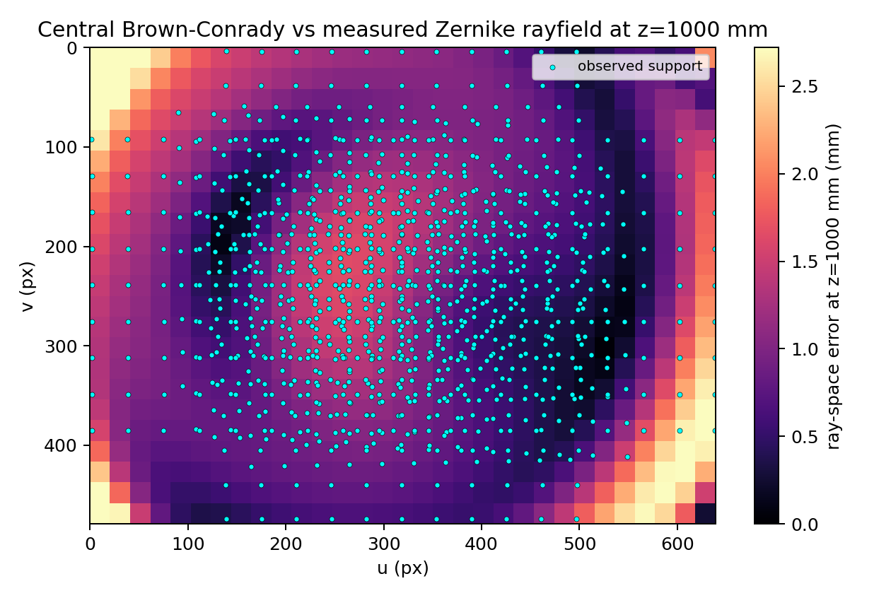
Fig. 30 Misspecified central Brown-Conrady residual against the measured Zernike rayfield. The model can bend directions but cannot reproduce the non-central pixel-dependent origin field.

This section illustrates a broader workflow: measure the rayfield first, then compare optical models in ray space. Les points 2D servent à mesurer le champ de rayons ; le champ de rayons sert ensuite à identifier l’optique.

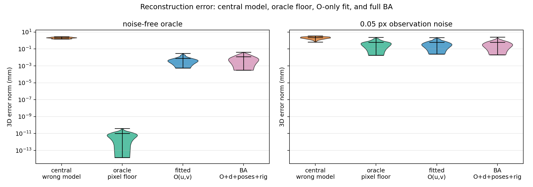
Fig. 31 3D reconstruction error distributions. The orange model is deliberately central and therefore wrong for this oracle; green is the oracle rayfield evaluated at the observed pixels; blue is the fitted O(u,v) field; purple is the experimental BA fit over O(u,v), d(u,v), board poses, and stereo rig.

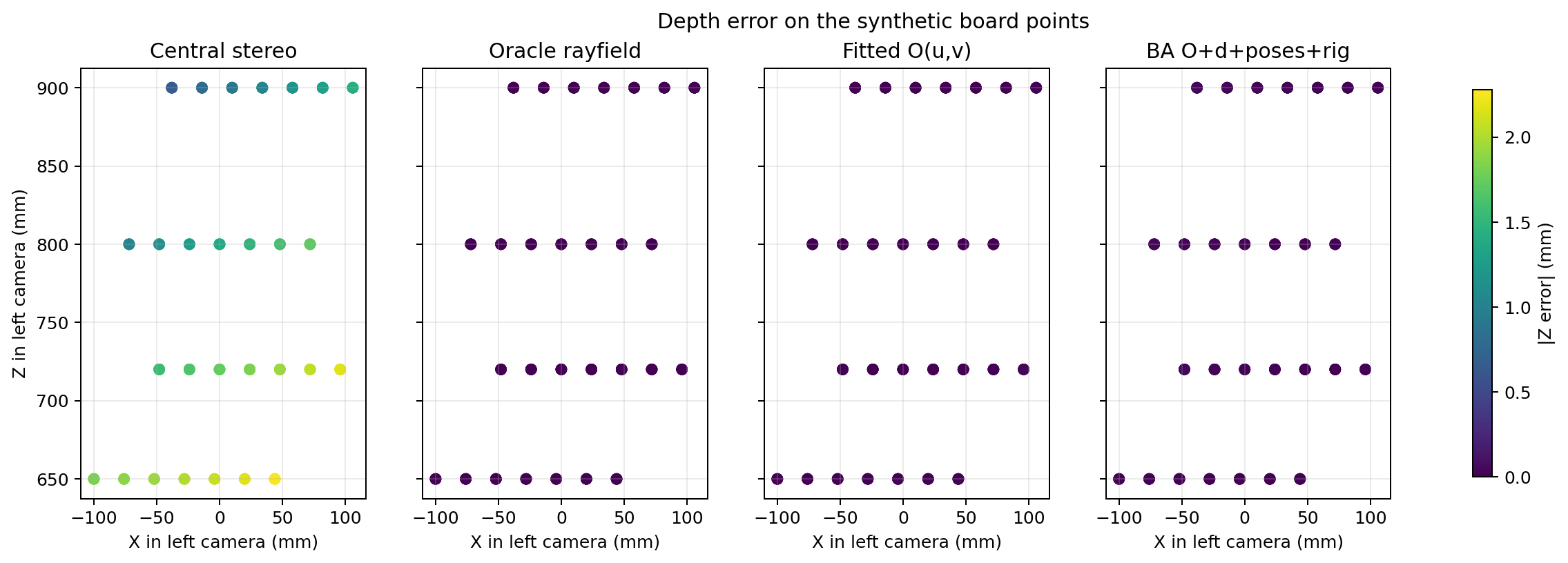
Fig. 32 Noise-free depth error. The central model shows a structured millimetre-scale depth bias; the oracle rayfield is numerically exact; the identified origin field reduces the error close to the fit residual scale.

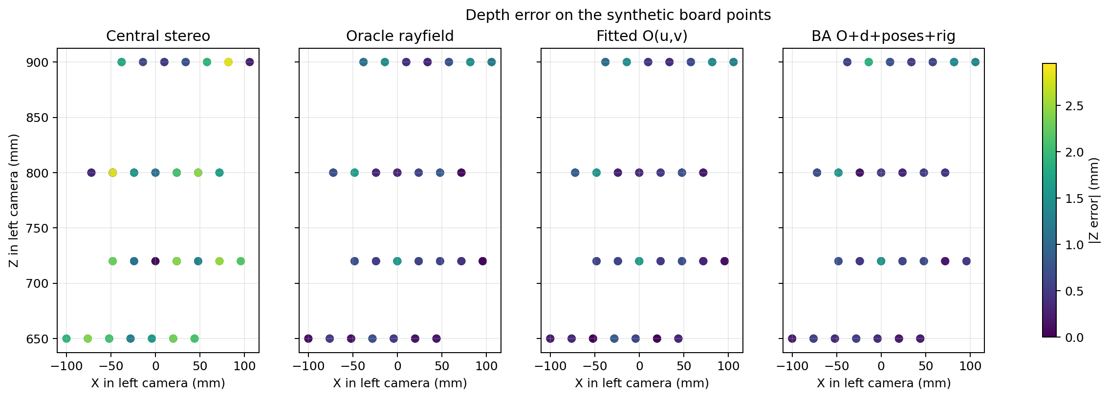
Fig. 33 Depth error with 0.05 px observation noise. The identified origin field and the experimental BA fit sit at the same scale as the oracle rayfield evaluated at noisy pixels.

Ray-field comparison against the oracle

Raw origins are not compared directly because the oracle uses the physical exit point I2, while the fitted model uses a transverse gauge. Instead, rays are intersected with two reference planes, z=100 mm and z=1000 mm, and the plane intersection error is summarized.

Case	L plane RMS (mm)	R plane RMS (mm)	Residual RMS (mm)	Residual P95 (mm)
Noise-free	0.831	0.621	0.00326	0.00547
0.05 px noise	1.520	0.802	0.0859	0.151

The heatmaps below show the single-plane error at z=1000 mm. Errors are small near the observed image region and grow near corners where the Zernike field is more weakly constrained by the synthetic board poses.

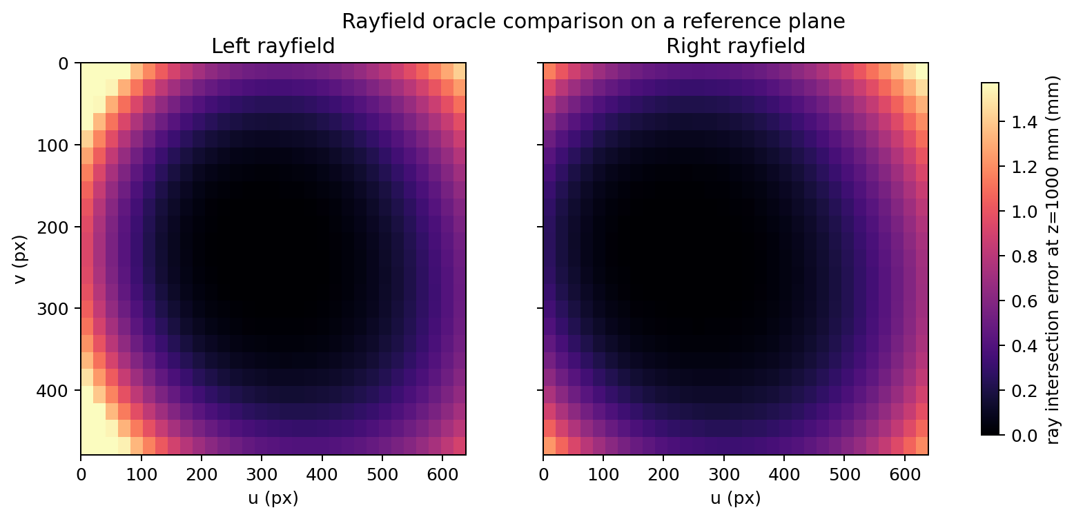
Fig. 34 Noise-free rayfield comparison on the z=1000 mm reference plane.

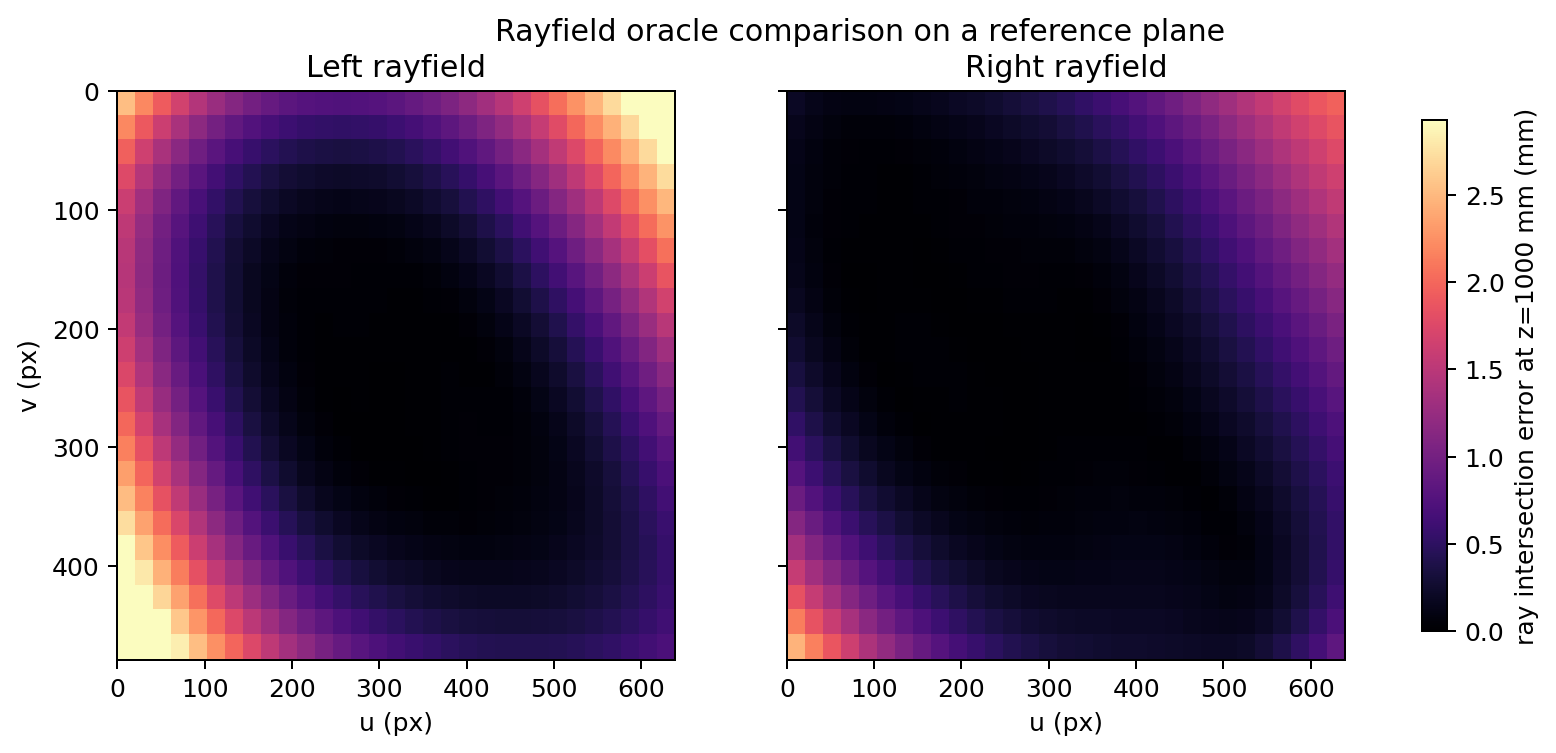
Fig. 35 Rayfield comparison on the z=1000 mm reference plane with 0.05 px observation noise.

Stereo ray consistency

The ray gap is the shortest distance between the two stereo rays before taking their midpoint. It is not the full 3D error, but it is a useful consistency diagnostic. In the noisy case, the oracle noisy-pixel reference and the fitted O(u,v) model and the BA O+d+poses+rig model have almost the same ray-gap distribution, which again indicates that the fit has reached the observation-noise scale.

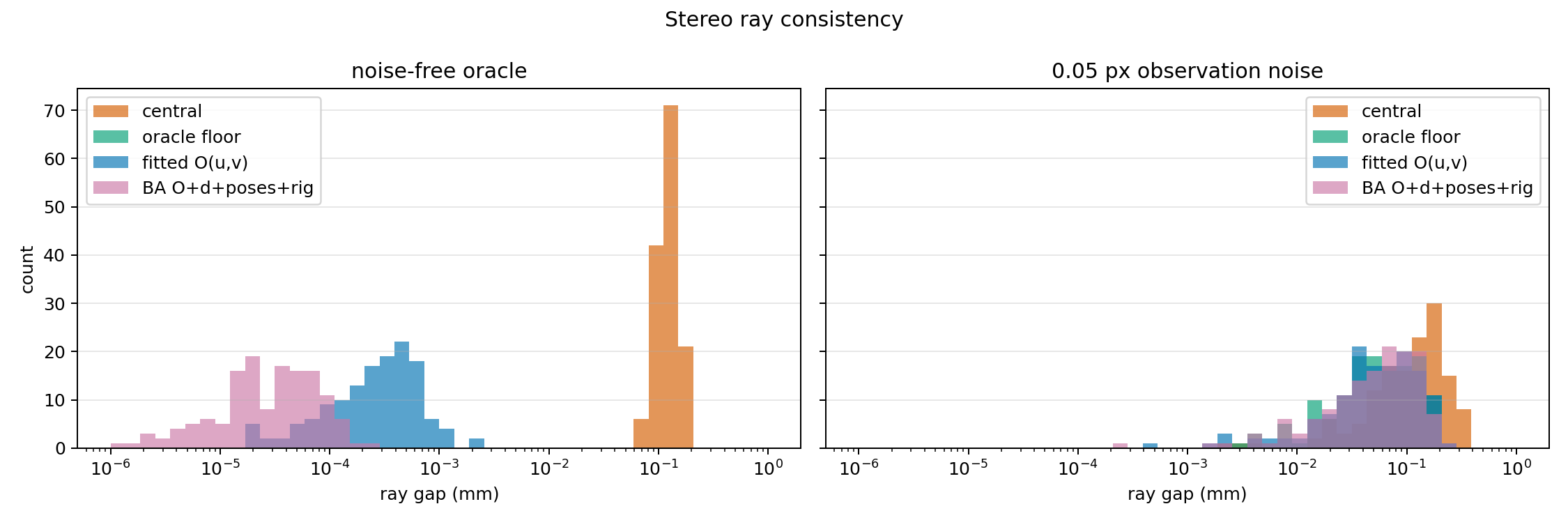
Fig. 36 Stereo ray gap distributions. The identified origin field makes the two rays geometrically more consistent than the central model, and approaches the oracle noisy-pixel reference in the noisy case.

Rendered-image front-end

The final check on this page uses the same non-central oracle to render actual ChArUco images. The render is intentionally not ideal: it includes vignetting, spatially varying blur, a mild illumination gradient, and sensor noise. OpenCV detects the ChArUco corners from those images, and the complete BA then optimizes O(u,v), d(u,v), board poses, and the stereo rig from the detected 2D points.

The rendered benchmark now follows a more realistic acquisition rule than the first smoke test: it uses 14 stereo poses (including 4 axis-aligned edge poses where roughly a quarter of the board extends outside the image) and a larger 12 x 9 ChArUco board. This is consistent with common calibration guidance: MathWorks recommends at least 10-20 images and a target covering at least about 20% of the image, and HALCON emphasizes varied poses covering the full field of view or measurement volume. The intent is not to tune a particular camera, but to avoid testing the full non-central BA with an obviously under-constrained tiny target.

This is a stricter test than the geometric oracle because the observations now include detector bias and rasterization effects. For that reason the table also reports an oracle detected floor: the exact parallel-plate rayfield is used for triangulation, but at the pixel positions returned by the 2D front-end. This isolates the error caused by image rendering and corner localization from the error caused by the non-central BA.

Two 2D front-ends are compared:

• OpenCV raw: the ChArUco corners returned by OpenCV are used unchanged;

• Ray2D refined: the detected ArUco marker corners are used to run the public rayfield_tps_robust planar refinement before the same non-central BA.

The 4 edge poses cover regions near each image border where a quarter of the board hangs outside the frame. ChArUco inner corners that lack an adjacent visible ArUco marker cannot be identified, so each edge frame contributes its own detected-corner subset. The per-frame corner counts therefore vary, and the table reports the minimum across all frames and the total pooled count.

Front-end	Frames	Min corners/frame	Total points
OpenCV raw	14	52	1139
Ray2D refined	14	52	1139

Front-end	Central RMS (mm)	Oracle RMS (mm)	BA RMS (mm)	Gain
OpenCV raw	4.266	3.250	3.159	1.35x
Ray2D refined	2.677	0.785	0.727	3.68x

The result changes the diagnosis. With raw OpenCV ChArUco corners, the oracle detected floor is already high (3.25 mm) and the complete BA only reaches 3.16 mm: the limiting factor is the raw detector/rasterization front-end. With the Ray2D planar refinement, the same rendered images and the same BA pipeline drop to 0.727 mm RMS, slightly below the oracle detected raw-pixel floor for the refined coordinates (0.785 mm). This is consistent with the geometric noise-floor estimate above and confirms that the non-central BA was not the main bottleneck in the raw rendered test.

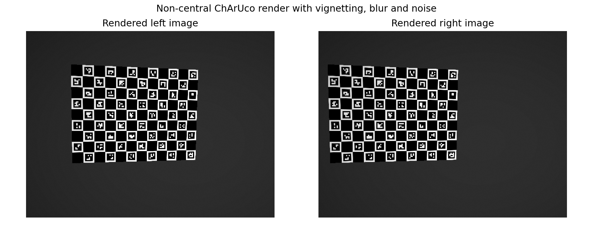
Fig. 37 Rendered stereo pair generated from the non-central parallel-plate rayfields. The image contains vignetting, spatially varying blur and sensor noise before OpenCV ChArUco detection.

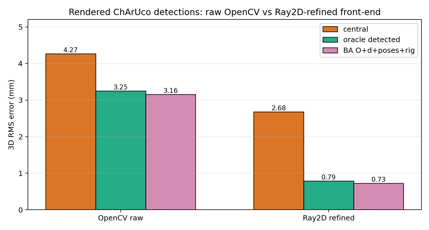
Fig. 38 Complete detected-image procedure. Raw OpenCV detections leave a high detector/rasterization floor. The Ray2D-refined front-end lowers that floor and lets the same full BA over O(u,v), d(u,v), poses and rig reach the expected sub-millimetre scale for this stereo geometry.

Generalization: held-out pose validation

A natural question after fitting is whether the identified rayfield memorises the training poses or genuinely represents the camera geometry. To answer this, make_parallel_plate_extended_dataset generates a 10-frame dataset (same oracle parameters as the default benchmark) and splits it into a training set and a hold-out set that is never seen by the BA.

	Frames	Points	Central RMS	Origin-field RMS
Training	0–7	280	2.16 mm	0.0002 mm
Hold-out (unseen)	8–9	70	2.08 mm	0.0003 mm
Ratio hold-out / training	—	—	—	1.5×

The origin-field trained on 8 frames reconstructs the 2 held-out poses at essentially the same accuracy (ratio 1.5×, well inside the 3× threshold used as the test criterion). This is expected: in the noise-free case a max_order=4 Zernike field can represent the parallel-plate lateral shift analytically over the observation domain, so there is no overfitting to observe.

The relevant test is test_holdout_poses_confirm_origin_field_generalises in tests/test_reconstruction_with_origin_field.py. It asserts:

• hold-out RMS < training RMS × 3.0 (no degradation relative to in-sample),

• hold-out RMS < 0.2 mm (absolute bound, well below the noise floor of a 0.05 px observation uncertainty which maps to ~0.7 mm at 700 mm depth).

The central model scores ~2.1 mm on both sets, confirming the bias is a systematic geometric effect (not pose-dependent noise), and that the origin field removes it on unseen poses as well as training ones.

Interpretation

This benchmark should not be read as a calibration of a glass plate. It answers a narrower question:

if the true stereo system is non-central, can StereoComplex identify a compact generic rayfield that improves 3D reconstruction?

For this oracle the answer is yes. The central model gives a millimetre-scale 3D bias even without noise, while the Zernike O(u,v) field removes that bias in the oracle case and generalises to held-out poses at comparable accuracy. Under 0.05 px observation noise, the fitted model reaches approximately the same RMS error as the exact oracle rayfield evaluated at noisy pixels, so the remaining error is consistent with stereo noise propagation.

Current scope limits:

• the default benchmark still reports the staged O(u,v)-only result because it isolates non-central identifiability;

• an experimental BA mode now optimizes O(u,v), d(u,v), board poses, and the stereo rig from image-coordinate observations;

• the rendered-image step now compares raw OpenCV ChArUco detections with the same detections after public rayfield_tps_robust planar refinement, then feeds both front-ends into the same complete BA;

• remaining validation should focus on real image sets.

The next experiment should use the same full procedure, keep the Ray2D front-end in the loop, and replace the synthetic oracle with real images:

parallel-plate oracle -> rendered images -> OpenCV detections -> Ray2D refinement
-> central initialization -> non-central BA over O,d,poses,rig
-> held-out 3D reconstruction metrics

Success should be judged against the oracle noisy-pixel floor reported above, not against zero error.