Physical CMO Model

This page answers: what physical assumptions define the shared-rig CMO model used by StereoComplex, and how it differs from a generic non-central polynomial surrogate.

This page defines the compact Common Main Objective (CMO) model implemented in stereocomplex.physics.CMOPhysicalStereoModel.

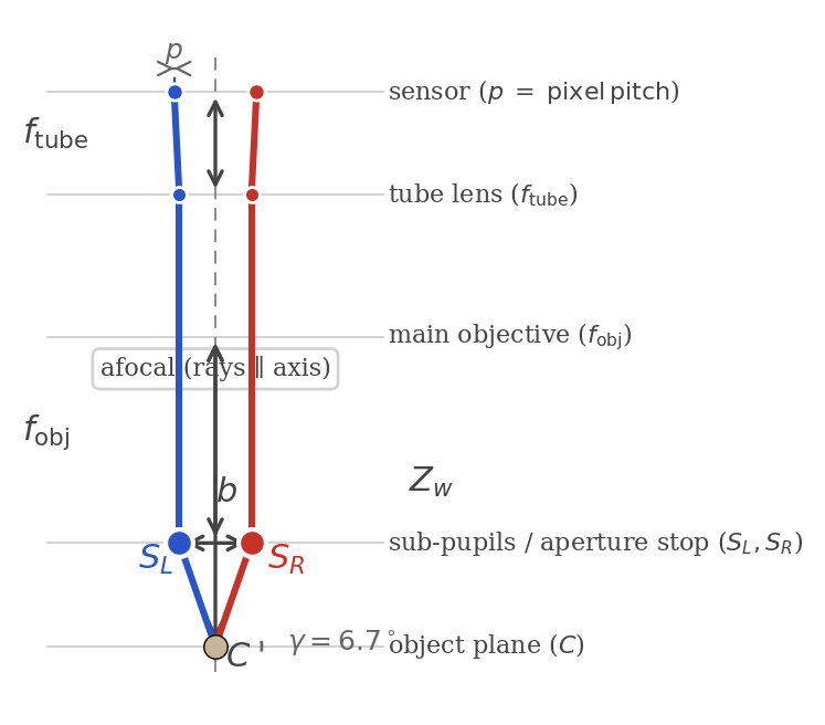
Fig. 39 Infinity-corrected CMO architecture. From top to bottom: sensor (\(p\)), tube lens (\(f_\mathrm{tube}\)), afocal space (rays parallel to axis), sub-pupils / aperture stop (\(S_L, S_R\), baseline \(b\)), main objective (\(f_\mathrm{obj}\)), working distance (\(Z_w\)), object plane (\(C\)). Chief rays (solid) converge at \(C\) through the shared objective.

It is not a full lens-design simulator. It is the object-side ray-space reduction of the CMO architecture: the sub-pupils, chief-ray convergence, and working-plane geometry are modelled explicitly, while the image-side optics (tube lenses, aperture stops, parallel afocal paths) are compressed into effective per-channel Brown-Conrady direction terms. Its goal is narrower: test whether a measured non-central rayfield is compatible with a shared-objective stereo microscope geometry.

Optical Assumption

A CMO stereo microscope is modeled as:

1. one common main objective;

2. two effective left/right sub-pupils separated by a baseline \(b\);

3. two tube-lens/sensor channels with identical pixel pitch;

4. optional per-channel effective direction distortion at the angular level.

The model enforces a structural CMO constraint: the left and right chief rays converge toward the working point on the main optical axis. This is different from the polynomial surrogate, where the two channels have independent effective origins and independent angular polynomial fields.

Parameters

The shared rig parameters are:

Parameter	Meaning
\(f_{\mathrm{obj}}\)	effective focal length of the common main objective
\(Z_w\)	working distance / chief-ray crossover plane
\(b\)	left/right sub-pupil separation
\(f_{\mathrm{tube}}\)	effective tube-lens focal length
\(c_x,c_y\)	shared principal point in pixels
\(p\)	pixel pitch in mm, fixed from the sensor datasheet
\(\theta_y\)	small global tilt around the vertical axis

Each channel also has Brown-Conrady coefficients

\[(k_1,k_2,p_1,p_2,k_3)_L, \qquad (k_1,k_2,p_1,p_2,k_3)_R.\]

The default optimized vector has 17 scalars. The pixel pitch is fixed from external sensor information, not optimized from ray geometry:

\[\theta = \left[ f_{\mathrm{obj}}, Z_w, b, f_{\mathrm{tube}}, c_x, c_y, \theta_y, \mathbf d_L, \mathbf d_R \right].\]

An optional aligned-sensor mode adds two effective degrees of freedom:

\[\delta c_{x,L}=-\frac{1}{2}\Delta c_x, \qquad \delta c_{x,R}=+\frac{1}{2}\Delta c_x,\]

and analogously for y. This keeps the gauge centered while allowing the two sensor principal points to be shifted relative to each other. In that mode the optimized vector has 19 scalars. The horizontal relative offset can correlate with the fitted sub-pupil baseline, so the most robust validation remains the rayfield residual and recovered shared geometry.

Ray Construction

For a pixel \((u,v)\) in channel \(c\in\{L,R\}\), first convert to tube-lens angular coordinates:

\[\alpha_x^d = \frac{(u-c_x)p}{f_{\mathrm{tube}}}, \qquad \alpha_y^d = \frac{(v-c_y)p}{f_{\mathrm{tube}}}.\]

The distorted angular coordinates are undistorted with the channel’s effective direction-distortion coefficients:

\[(\alpha_x,\alpha_y) = D_{\mathrm{Brown}}^{-1} \left( \alpha_x^d,\alpha_y^d; k_1,k_2,p_1,p_2,k_3 \right).\]

Effective vs physical distortion

The five per-channel coefficients are Brown-Conrady-like coefficients applied to normalized angular coordinates. They define an effective parameterization \mathcal D_c, intended to absorb residual direction errors from the tube lens, relay optics and main objective. They should not be read as a derivation from a specific Seidel or wavefront-aberration model.

Let \(s_L=-1\) and \(s_R=+1\). The effective sub-pupil point is

\[S_c= \left( s_c\frac{b}{2}, 0, Z_w-f_{\mathrm{obj}} \right)^T.\]

The pixel selects a point on the working plane:

\[P_c(u,v)= \left( Z_w\alpha_x, Z_w\alpha_y, Z_w \right)^T.\]

The ray is the line through \(S_c\) and \(P_c\):

\[\mathcal R_c(u,v)= \left( S_c, \frac{P_c(u,v)-S_c}{\|P_c(u,v)-S_c\|} \right).\]

For the central pixel, \(P_c=(0,0,Z_w)^T\). The chief-ray angle is therefore

\[\gamma=\arctan\left(\frac{b}{2f_{\mathrm{obj}}}\right),\]

and both channels cross the optical axis at the working plane. This chief-ray constraint is the main geometric difference between the physical CMO and a pair of independent non-central polynomial channels.

Identifiability

From ray geometry alone, \(f_{\mathrm{tube}}\) and pixel pitch \(p\) appear through the ratio \(p/f_{\mathrm{tube}}\). They are not separately identifiable unless one of them is fixed by external information. StereoComplex therefore fixes pixel_pitch_mm from the sensor specification and optimizes f_tube_mm; the identifiable angular scale remains $p/f_{\mathrm{tube}}`.

Similarly, strong Brown radial coefficients can be correlated if the observed field of view is narrow. The robust validation quantities are:

• ray-space RMS against the measured Zernike field;

• chief-ray convergence and effective CMO baseline;

• recovered working plane and sub-pupil geometry;

• pose consistency in the CMO bundle-adjustment benchmark.

Relation To The Polynomial Surrogate

The existing NonCentralPolynomialChannelModel is better described as a generic non-central polynomial channel surrogate. It is useful because it can fit many smooth rayfields, including CMO-like ones, but it does not encode the shared main-objective constraints.

The physical CMO model is less flexible but more interpretable. On a true CMO oracle, it achieves sub-micron RMS with 17 shared parameters. The polynomial surrogate can also represent the CMO rayfield (with free origin_z and a constant aberration term), but requires ~36 independent parameters. The BIC gap is therefore driven by parametric compactness: the physical CMO wins because it encodes the correct shared-objective structure, not because it is the only model that can explain the rayfield.

Real microscope mapping

The two model families — physical CMO shared-rig and non-central polynomial surrogate — correspond to real commercial stereo microscope architectures. Use this table to decide which candidate is appropriate for your instrument.

Physical CMO shared-rig model

Use when the instrument has one common main objective with two parallel afocal zoom paths and a shared sub-pupil baseline.

Manufacturer	Model	Zoom ratio	Max NA	Notes
Leica	M205 C / M205 A	20.5:1	0.35	100 % apochromatic CMO; FusionOptics asymmetric per-channel resolution/depth
Evident / Olympus	SZX16	16.4:1	0.30	Galilean CMO; 65.7:1 effective with objective nosepiece; WD up to 141 mm
Zeiss	SteREO Discovery.V20	20:1	~0.35	Motorized eZoom CMO; up to 1000 lp/mm
Zeiss	SteREO Discovery.V12	12:1	—	Same modular CMO platform as V20
Nikon	SMZ25	25:1	0.312	“Perfect Zoom System” CMO; 0.63×–315× total magnification

Even within the CMO family, real instruments can introduce per-channel asymmetries:

• Leica FusionOptics deliberately gives the left and right channels different resolution and depth-of-field characteristics. This may produce measurably different per-channel distortion that the share_principal_point=False (19-parameter) mode is designed to absorb.

• Tube-lens and relay variations between the two channels can add per-channel effective distortion beyond the shared objective.

Non-central polynomial surrogate

Use when the instrument has independent optical paths per channel — no shared main objective, or unknown/heterogeneous optics.

Manufacturer	Model	Zoom ratio	Notes
Zeiss	Stemi 508	8:1	Greenough; 35° convergence angle; WD up to 287 mm
Leica	Ivesta 3	9:1	Greenough with FusionOptics; integrated 12 MP camera; WD up to 122 mm
Evident / Olympus	SZ61	6.7:1	Greenough; entry-level inspection stereo microscope

Greenough microscopes are the canonical case: two completely separate objective lenses, one per channel, typically angled inward (convergent axes). Each channel has its own entrance pupil, and there is no shared objective geometry.

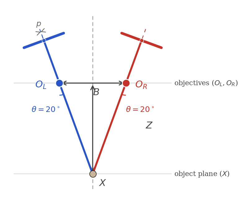
Fig. 40 Greenough stereo microscope. Two independent objectives \(O_L, O_R\) with convergent optical axes tilted by \(\pm\theta\) from the vertical. Each channel has its own tilted sensor (pixel pitch \(p\)) and its own optical axis. There is no shared main objective — contrast with the CMO diagram above. Baseline \(B\) and working distance \(Z\) are annotated.

Other architectures that fall in the polynomial surrogate category:

Architecture	Why non-central, non-CMO
Industrial stereo with per-channel windows or prisms	Each camera’s protective window, beamsplitter, or right-angle relay adds per-channel refractive distortion (astigmatism, lateral shift) not shared between channels.
Scheimpflug / tilted-sensor stereo	Each sensor has a different orientation relative to its lens, producing asymmetric projections that cannot be modelled by CMO or Greenough alone. Common in line-scan stereo for web inspection.
Stereo endoscopes / borescopes	Single objective housing with two relay channels and separated sub-pupils (3–5 mm baseline); GRIN lenses or fiber relays. Wide-angle optics produce strong non-central effects.
Dual-camera rigs with unknown or asymmetric optics	Any setup where the two cameras have different lenses, filters, or mounts. The polynomial surrogate is the safe fallback.

Decision flow

Does the instrument have a single shared main objective?
  ├── Yes → physical CMO shared-rig model (17 or 19 params)
  │         Also test the polynomial surrogate as a fallback:
  │         if it wins BIC, the shared-objective hypothesis is
  │         not supported by the rayfield data.
  └── No  → non-central polynomial surrogate (34 params total)
            Also test central Brown-Conrady and inclined-plate
            candidates to rule out simpler explanations.

References

• Olympus US 7,564,619, “Stereoscopic microscope”, 2009.

• Wang et al., “Calibration of a stereo microscope based on non-coplanar feature points”, Optics and Lasers in Engineering, 134, 2020.

• Schreier, Garcia and Sutton, “Advances in light microscope stereo vision”, Experimental Mechanics, 44(3), 278-288, 2004.

• Pan, Wang and Cheng, “High-accuracy 3D shape and deformation measurements with a CMO stereo microscope”, Optics Express, 22(15), 18373-18387, 2014.