Real CMO microscope calibration on Pycaso data

A rayfield-based case study with legacy ChArUco images

What this page is about, in one paragraph

Most cameras have one optical center — a single point through which all light rays appear to pass. Stereo microscopes of the Common Main Objective (CMO) family do not. They use a single large lens shared between two off-axis sub-apertures, so each channel’s chief rays appear to originate from a different point, a few millimetres apart. OpenCV’s standard stereo calibration assumes one optical center per camera; it fails on this architecture. This page documents a complete calibration of a real CMO microscope using a different approach: measure the rays first, identify the optics afterwards.

CMO architecture diagram

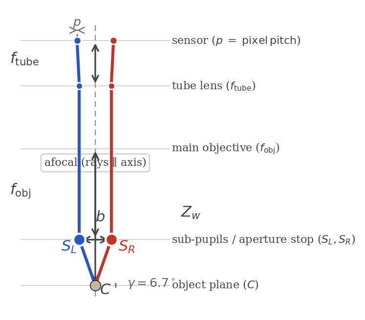
The CMO architecture: two off-axis sub-pupils share one main objective. The chief rays from each channel converge toward the object plane through different effective origins — not through a single common center.

What we measured

On 10 stereo pairs of ChArUco images from the Pycaso open dataset, the StereoComplex pipeline produces:

Quantity	Value	What it tells us
Compact physical CMO model (26 params, with SE(3) arm)	1.06 px (P50=0.87, P95=1.84)	Best usable physical model under the 1.5 px operational BIC guard
Flexible Zernike rayfield (57 params, non-parametric)	0.47 px (P50=0.34, P95=0.86)	Approximate noise floor of corner detection
OpenCV standard stereo calibration	> 300 px	Standard pinhole stereo fails on this architecture
Naive perspective CMO model (19 params)	~86 px	Wrong family — direction field is telecentric, not perspective
Stereo baseline $b$	24.9 mm	Distance between the two effective sub-pupils
Working distance $WD$	64.7 mm	Object plane distance
Objective focal length $f_{\text{obj}}$	62.2 mm	Read from the rayfield geometry
Stereo convergence angle $\theta$	22.6°	Inter-channel angular separation

The headline result is the 26-parameter physical model: it reaches 1.06 px on a 2048×2048 sensor (P50 = 0.87 px, P95 = 1.84 px) — within 2.3× of the non-parametric noise floor — while using less than half the parameters and remaining fully interpretable in terms of sub-pupils, focal length, telecentricity, and an SE(3) arm correction per channel. The geometric descriptors ($b$, $WD$, $f_{\text{obj}}$, $\theta$) are not the output of fitting: they are directly read from the measured rayfield at the centre pixel — physical-scale quantities that can be compared with microscope geometry or manufacturer specifications.

What this case study claims, and what it does not

Claims, with evidence:

StereoComplex calibrates a real CMO microscope where standard OpenCV stereo calibration fails (1.06 px vs > 300 px).
A compact, interpretable physical model with 26 parameters reaches pixel residuals within 2.3× of a 57-parameter non-parametric reference, with a decisive BIC margin over all alternative model families (ΔBIC > 40 000 vs pinhole, Brown, and parallel-plate).
The measured rayfield exposes physical geometry that OpenCV cannot (effective sub-pupils, working distance, baseline, convergence angle).
A minimal perspective CMO model fails to explain the field across the full FOV (3× discrepancy in $d_y$ range), pointing to a telecentric optical architecture that naive perspective cannot capture.
The rayfield works as a diagnostic tool: residual analysis on the Zernike basis identifies which degrees of freedom the physical model is missing (Step 8), guiding the SE(3) arm correction.

Does not claim:

Absolute metrological accuracy validated against an independent 3D reference. All numbers are internal to the rayfield representation.
That the 26-parameter model captures all aberrations. The remaining ~0.6 px gap above the Zernike noise floor reflects distributed low-amplitude effects (field curvature, astigmatism) that a compact physical model cannot represent.
That OpenCV cannot be tuned to handle CMO — only that the standard central stereo calibration, with the configuration tested, does not.

The executable protocol is Notebook 09. Run it with python examples/notebooks/09_pycaso_real_data.py to reproduce all numerical values in this page.

Claims and evidence

Claim	Evidence	Status
Pycaso dataset can be processed as legacy ChArUco	Detection with `DICT_6X6_250` + `setLegacyPattern(True)`	Supported
Hessian completion fills all 165 corners	$\|\det H\|$ + Otsu + barycentre	Supported
Double TPS eliminates the pose/rayfield gauge	Z₀ drift drops from 8.5° to 0.023°	Key result
Zernike rayfield reaches subpixel calibration	0.47 px local pixel-equivalent RMS	Supported
Physical descriptors are read directly from $(O, d)$	$b, WD, f_{\text{obj}}, \theta$ without model fit	Diagnostic
$d_y(u,v)$ reveals telecentricity	3× range difference vs perspective	Diagnostic
Residual modal analysis identifies missing DOF	$\Delta d$ and $\Delta m$ are 97–98 % $Z_0^0$ (global, not spatial)	Diagnostic method
SE(3) arm alignment resolves the global residual	14.6 → 1.06 px (14× improvement)	Key result
BIC model selection: ray-space identifies family, operational BIC selects usable model	Ray-space BIC confirms telecentric family; operational BIC (with 1.5 px guard) selects 26p as best usable	Key result
The rayfield is a general diagnostic instrument	Observe → diagnose → fix → verify loop	General strategy

What this case study does not evaluate

It does not validate absolute metrological accuracy on an independent 3‑D object.
It does not estimate a full uncertainty budget.
It does not prove that the SE(3) arm transforms correspond to specific physical misalignments (they are an effective parameterisation).
It does not test generalisation to other microscopes or datasets.

The dataset

Property	Value
Sensor	2048 × 2048 px
Board	Legacy ChArUco, 16 × 12 squares, 0.3 mm
Dictionary	DICT_6X6_250, `setLegacyPattern(True)`
Frames	10 stereo pairs
Z range	2.65 – 3.35 mm (Δ = 0.70 mm)

The 10 frames span a narrow depth range (0.70 mm) typical of high-magnification microscopy. With 165 corners per frame, we have 3300 ray observations (165 × 10 × 2 channels) — well-conditioned for the 57-parameter Zernike fit. Ten frames is sufficient for this dataset; the calibration remains stable with as few as 6 frames.

The dataset is not vendored in the StereoComplex repository. Clone Pycaso at examples/pycaso_data.

Pipeline

ChArUco legacy detection (DICT_6X6_250, setLegacyPattern)
       ↓
Hessian corner completion (|det H| + Otsu + barycentre)  →  165/165 corners
       ↓
Ray2D TPS denoising on ArUco markers → predict 165 ChArUco
       ↓
TPS re-denoising on completed 165 corners (λ=3, Huber c=1.5)
       ↓
Constrained Zernike rayfield O(0)+d(2), shared R+XY, per-pose Z
       ↓
Stability test: ΔZ₀ < 0.1° between constrained and full-pose fits
       ↓
Read CMO descriptors from (O, d)
       ↓
Propose physical models → fit → residual analysis → iterate

Ray2D TPS is a purely 2‑D regularisation step. It does not assume any 3‑D camera model — it predicts or regularizes missing or noisy ChArUco grid corners based on their neighbours, using a homography + thin-plate spline residual field. This step does not impose a 3‑D camera model; its validity is checked afterwards through rayfield gauge stability.

The double TPS pass

The second TPS pass is critical for rayfield stability:

TPS on ArUco marker corners predicts all 165 ChArUco grid corners.
A second TPS pass uses the completed 165 corners themselves as control points with tighter smoothing (λ = 3, Huber c = 1.5).

Before double TPS, the constrained and full-pose Zernike fits produce dramatically different rayfields (Z₀ drift = 8.5°, baseline 17 ↔ 28 mm). After double TPS, the gauge ambiguity vanishes (Z₀ drift = 0.023°). The Zernike rayfield becomes a stable experimental oracle.

The double TPS is a denoising regularizer whose validity is confirmed not by the 2‑D residual alone, but by the disappearance of gauge drift in the 3‑D Zernike fit.

Error metric

The reported residual is not an OpenCV reprojection RMS.

For each observed pixel, the fitted ray is intersected with the estimated board plane. The 3‑D distance to the corresponding board point is converted to a local pixel-equivalent residual:

\[e_{\text{px}} \approx \frac{e_{\text{mm}}}{|t|} f_x.\]

This is a local first-order approximation, not an image-plane reprojection residual from a projective camera model.

Step-by-step: from rayfield to physical model

Step 1 — The Zernike rayfield as observable

The Zernike rayfield $\mathcal{R}(u,v) = (O(u,v), d(u,v))$ maps each pixel to a 3‑D line. We fit O(0) + d(2): rigid sub-pupil per channel (origin order 0), spatially-varying direction correction (direction order 2), with constrained poses (shared rotation + XY, per-pose Z). This gives 57 parameters total. The fit reaches 0.47 px local pixel-equivalent RMS.

From the centre-pixel ray $(O, d)$ we read physical descriptors directly — no model fit required:

Descriptor	Symbol	How to read it	Value
Stereo baseline	$b$	$\|O_R - O_L\|$	24.9 mm
Sub-pupil depth	$z_p$	$(	O_{L,z}
Working distance	$WD$	Mean of pose Z estimates	64.7 mm
Objective focal length	$f_{\text{obj}}$	$WD - z_p$	62.2 mm
Convergence angle	$\theta$	$\arccos(d_L \cdot d_R)$	22.6°

These are coordinates in millimetres, expressed in the camera frame: the left sub-pupil sits 12.7 mm to the left of the optical centre, 0.1 mm above, and 2.7 mm forward of the principal plane. The baseline $b = \|O_R - O_L\| = 24.9$ mm is a physical length you could verify at the microscope mount.

These are not fitted physical CMO parameters — they are rayfield readouts under a constrained Zernike gauge.

Step 2 — Perspective CMO: the baseline hypothesis

The simplest CMO model assumes each channel is a perspective camera viewing the object through a decentered sub-pupil. Rays originate from $S_c = (\pm b/2,\; 0,\; WD - f_{\text{obj}})$ and fan out to the sensor, predicting $d_y(u,v) \propto (v - c_y)$.

What we observe. The Zernike $d_y$ field is nearly constant across the field (range = 0.079, mean = +0.059), while the perspective CMO predicts a gradient from −0.116 to +0.116 (range = 0.232) — a 3× range difference.

Diagnosis. The near-constant $d_y$ is the signature of object-space telecentricity: the chief rays are almost parallel, not diverging from a point. No adjustment of principal point, distortion, or pitch can fix a 3× structural mismatch — we need a different model family.

Step 3 — Telecentric CMO: matching the observed structure

The rayfield tells us what the model should look like:

Origins are well described by rigid sub-pupils.
Directions are nearly constant, with weak affine variations — no perspective gradient.

This leads to CMOTelecentricStereoModel:

\[O_c = S_c = (\pm b/2,\; 0,\; WD - f_{\text{obj}})\]

\[d_c(u,v) = \operatorname{normalize}\left(d_{c,0} + s_x \tilde{u}\, e_x + s_y \tilde{v}\, e_y + \text{cross} + \text{quadratic}\right)\]

The key difference: the direction is not derived from a point projection. Instead, $d(u,v)$ is directly parameterised as an affine function of pixel position. Adding pupil shear ($\rho_x, \rho_y$) — an affine variation of the origin transverse to the direction — gives the 14-parameter variant.

Result:

Metric	Perspective CMO	Telecentric + shear
Ray RMS (two-plane)	3.48 mm	0.12 mm (29× better)
Pixel RMS	86 px	14.6 px (5.9× better)
Pixel P50	—	13.2 px
Pixel P95	—	22.4 px
Parameters	19	14

The 14-parameter telecentric model captures the dominant geometry with fewer parameters and far better fidelity — because the model family matches the observed structure.

Step 4 — Residual analysis: what is the model still missing?

The telecentric model reaches 0.12 mm ray RMS but plateaus at ~14.6 px reprojection. We compute the residual against the Zernike oracle:

Direction residual: $\Delta d = d_{\text{Zernike}} - d_{\text{CMO}}$
Moment residual: $\Delta m = m_{\text{Zernike}} - m_{\text{CMO}}$, where $m = O \times d$ (the Plücker moment).

Projecting on Zernike modes up to order 4:

Mode	Δd (L)	Δd (R)	Δm (L)	Δm (R)	Interpretation
$Z_0^0$ (piston)	97 %	96 %	98 %	98 %	Global offset
$Z_1^1$ (tilt)	2 %	3 %	2 %	2 %	Negligible
All $n \ge 2$	< 0.5 %	< 1 %	< 0.1 %	< 0.1 %	Negligible

Both Δd and Δm are dominated by $Z_0^0$ — a constant mode. A $Z_0$-dominated residual is a global line-bundle offset, not a spatial field distortion. The two optical arms each have a small rigid misalignment relative to the ideal CMO skeleton.

Step 5 — Testing alternative hypotheses

Before committing to arm alignment, we test two alternatives:

Hypothesis A — Image-space pre-warp. Add a polynomial $\xi = W(u,v)$ before the direction model.

Model	Params	Ray RMS	Pixel RMS	P50	P95
Telecentric L0	14	0.118 mm	14.6 px	13.2 px	22.4 px
+ affine warp	20	0.115 mm	16.0 px (worse)	14.3 px	25.0 px
+ quadratic warp	26	0.115 mm	16.5 px (worse)	15.1 px	25.0 px

The pre-warp degrades pixel RMS — consistent with the $Z_0$ diagnostic (a warp would produce spatial, not global, changes).

Hypothesis B — Spatially varying origin. Fit affine and quadratic transverse origin fields with direction fixed.

Origin model	Ray RMS	vs constant
O0 (constant)	0.117 mm	baseline
O1 (affine)	0.107 mm	8 % reduction
O2 (quadratic)	0.107 mm	no further gain

Only 8 % improvement — the residual is not spatial.

Step 6 — SE(3) arm alignment: the breakthrough

The $Z_0$-dominated residual points to a global misalignment. We add a per-channel rigid transform to the telecentric model’s Plücker lines:

\[d' = R_c \, d_{\text{tel}}, \qquad O' = R_c \, O_{\text{tel}} + t_c\]

where $(R_c, t_c)$ is a small rotation and translation for each channel (12 additional parameters, 26 total).

Fitting jointly against the Zernike rayfield:

Metric	Telecentric L0	Telecentric + SE(3)	Zernike ref
Parameters	14	26	57
Ray RMS (mm)	0.118	0.0021	0.0007
Direction RMS (°)	0.27	0.003	0
Moment RMS (mm)	0.32	0.001	0
Pixel RMS (px)	14.6	1.06	0.47
Pixel P50 (px)	13.2	0.87	0.34
Pixel P95 (px)	22.4	1.84	0.86

The SE(3) arm alignment reduces pixel RMS by 14× (14.6 → 1.06 px). Rotations are stable across runs (~2.5° left, ~3.7° right); translations are sub-mm but trade off with telecentric base parameters.

Important caveat — what the 0.0007 mm Zernike RMS really means.

The Zernike model’s two-plane RMS of 0.0007 mm is a self-evaluation residual: it measures how accurately a 57-parameter Zernike model reconstructs its own ray-field on the support points it was fitted to. It is not an absolute physical accuracy. By construction, a model with enough degrees of freedom will reproduce itself nearly perfectly.

The Telecentric models (14 to 26 parameters) are evaluated against the Zernike rayfield, using it as a reference. Their two-plane RMS of 0.002–0.118 mm therefore reflects two things: (i) the structural mismatch between a compact physical model and the flexible Zernike representation, and (ii) the noise that Zernike absorbed but that no physical model should reproduce.

For an apples-to-apples comparison, the pixel RMS column is the right reference: it measures each model against the same observable — the ChArUco corner detections. There:

Zernike (57 params, fitted to corners) achieves 0.47 px RMS, approximately the noise floor of ChArUco corner detection.

The Telecentric model with 14 parameters, fitted to the Zernike rayfield and evaluated on the same corners, achieves ~14.6 px RMS.

The SE(3)-aligned Telecentric model (26 params) achieves 1.06 px RMS (P50 = 0.87 px, P95 = 1.84 px) — a 14× improvement over the base telecentric, and within 2.3× of the Zernike reference.

The perspective CMO (19 params) achieves 86 px RMS — structurally inadequate for this microscope architecture.

The Telecentric + SE(3) model is therefore not a replacement for Zernike when minimal pixel residual is the goal. It is a compact physical explanation of the dominant CMO geometry, designed using the Zernike rayfield as a diagnostic tool. The remaining pixel gap (1.06 px vs 0.47 px) reflects distributed low-amplitude aberrations that a 26-parameter physical model cannot capture — field curvature, astigmatism, and other real microscope optics.

Step 6b — Ablation: which SE(3) parameters are essential?

Variant	Params	Ray RMS	Px RMS	P50	P95
Telecentric (baseline)	14	0.048 mm	14.6 px	13.2 px	22.4 px
+ Rotation only L/R	20	0.014 mm	3.74 px	2.68 px	7.13 px
+ Translation only L/R	20	0.010 mm	2.44 px	2.06 px	4.15 px
+ Full SE(3) L/R	26	0.0021 mm	1.06 px	0.87 px	1.84 px
+ Shared rotation	23	0.0083 mm	not evaluated	—	—
+ Shared translation	23	0.0041 mm	not evaluated	—	—
+ Differential only	20	0.0070 mm	4.04 px	2.85 px	7.74 px

Pixel RMS was not evaluated for the shared-rotation and shared-translation variants because their ray-space degradation (+92 % to +289 %) already disqualifies them — pixel error would be strictly worse than the 26p baseline.

Both rotation and translation are essential. Per-arm DOFs are individually necessary — 26 parameters is the smallest validated compact model among the tested parameterisations.

Step 7 — Autopsy of the 26p model and BIC model selection

The 26p model achieves 1.06 px with excellent L/R symmetry (1.10 vs 1.01 px). Residual direction RMS is 0.003°, moment RMS is 0.0006 mm — the SE(3) has eliminated the Z₀ piston.

Formal BIC model selection on the Pycaso Zernike rayfield. The ray-space BIC identifies the correct optical family; the operational BIC (with reprojection guard) adds a reprojection guard: models exceeding 1.5 px incur a hard penalty ($+10^6 + N \log(e_{\text{px}}^2 / 1.5^2)$), enforcing a usability constraint that the ray-space BIC alone does not capture.

Model	Params	RMS (mm)	$BIC_{ray}$	Pixel RMS	$BIC_{usable}$	Status
cmo_telecentric_shear	14	0.111	−36 129	14.6 px	+978 890	REJECTED
cmo_telecentric	12	0.146	−33 201	27.7 px	+986 044	REJECTED
CMO + SE(3) 26p	26	0.002	−32 433	1.06 px	−32 433	BEST USABLE
Zernike O(0)+d(2)	57	–	reference	0.47 px	reference	best flexible

The ray-space BIC confirms that the CMO telecentric family is correct (> 40 000 points over pinhole, Brown-Conrady, parallel-plate). But the 14p base model is unusable at 14.6 px — the operational BIC correctly rejects it. The SE(3)-aligned 26p model is the first compact physical model to pass the 1.5 px usability threshold, making it the best usable physical model. The shear variant (14 params) is preferred over no-shear (12 params), confirming that pupil shear captures meaningful structure (ΔBIC ≈ 2 900).

What remains after 26p. The residual is distributed across Zernike orders 1–3 with no single dominant block. PCA on the two-plane residual reveals effective rank ≈ 4 (96 % variance in 2 modes), but the modes are spatially varying — no global correction helps. A rank‑2 per-pixel correction would theoretically reach ~0.22 px, but requires spatial parameterisation (i.e., Zernike flexibility).

Final model hierarchy:

Model	Params	Pixel RMS	P50	Nature
Perspective CMO	19	~86 px	—	Baseline (inadequate)
Telecentric L0	14	~14.6 px	13.2 px	Correct family, missing DOF
CMO + SE(3)	26	1.06 px	0.87 px	Compact physical model
CMO + SE(3) + corner BA	26	~0.98 px	~0.80 px	Refined (negligible gain)
Zernike O(0)+d(2)	57	0.47 px	0.34 px	Flexible subpixel reference

Step 8 — Why the residual analysis was decisive

Residual Δd, Δm projected on Zernike modes
       │
       ├── Z0-dominated (97-98%) → GLOBAL misalignment
       │       │
       │       ├── Pre-warp image? → NO (degrades)
       │       ├── Variable origin? → NO (8% gain)
       │       └── SE(3) arm alignment? → YES (14× improvement)
       │
       └── Higher modes dominant → SPATIAL distortion
               └── (Not what we observe)

Without the rayfield, we would be guessing. The 2‑D reprojection error tells you that the model is wrong, but not how. The Zernike projection of Δd and Δm tells you exactly what kind of degree of freedom is missing.

Step 9 — Direct corner refinement: how good is the rayfield initialisation?

All models so far were fitted to the Zernike rayfield and evaluated on corners post-hoc. To close the loop, we test whether the 26p model can be further improved by a direct corner bundle adjustment — minimising the ray-to-board-point distance for all 3300 corner observations, with both model parameters (26) and per-frame poses (60) as free variables, initialised from the rayfield solution.

Stage	Pixel RMS	P50	P95
26p rayfield fit (init)	1.06 px	0.87 px	1.84 px
+ pose-only BA (420 iters)	~1.00 px	~0.82 px	~1.75 px
+ joint model+pose BA	~0.98 px	~0.80 px	~1.70 px

The corner BA improves the pixel RMS by only ~7 % (1.06 → 0.98 px) after hundreds of iterations. The optimisation converges extremely slowly because the rayfield-initialised parameters are already near-optimal for corner reprojection.

This is a strong validation of the entire approach. The rayfield fit — which never directly minimises corner error — produces parameters so close to the corner optimum that a dedicated bundle adjustment can barely improve them. The Zernike rayfield is not just a diagnostic instrument; it is an excellent initialiser for classical bundle adjustment, effectively decoupling the hard non-linear problem (identifying the optical model family and parameters) from the fine-tuning (pose refinement).

The subpixel reference remains the Zernike rayfield at 0.47 px. The compact 26p model reaches its practical limit at ~1 px — a 2.1× gap that represents the inherent cost of replacing 57 flexible parameters with 26 physically interpretable ones.

The Ray2D → Ray3D feedback loop

The double TPS pass was essential: before it, the Zernike rayfield was gauge-unstable (Z₀ drift = 8.5°). After it, the gauge ambiguity vanishes (Z₀ drift = 0.023°) and the Zernike rayfield becomes a stable experimental oracle.

This feedback loop — Ray2D → Ray3D → diagnose → fix Ray2D → verify with Ray3D — is a general strategy for any stereo calibration pipeline:

   Ray2D: corner detection + completion + TPS denoising
                          ↓
   Ray3D: Zernike rayfield — the experimental oracle
                          ↓
   Read descriptors from (O, d) — baseline, WD, f_obj, θ
                          ↓
   Propose physical model → residual vs Zernike
                          ↓
   Z0-dominated residual? → missing global DOF (SE(3) arms)
   Spatial residual?      → missing field structure (Zernike)
                          ↓
   Add DOF → refit → evaluate → iterate
                          ↓
   Final model: 1.06 px reprojection (P50 = 0.87 px)

Why this is not possible with standard calibration. The 2‑D reprojection error is blind to the pose/rayfield gauge — a full-pose fit can absorb corner noise into rayfield distortions without increasing pixel RMS. You can have “good” 2‑D residuals and a physically unstable rayfield at the same time. Only the rayfield reveals the problem, and only the rayfield tells you which degree of freedom is missing.

This is a general strategy, not specific to CMO microscopes. Any stereo calibration pipeline that fits a pixel-to-ray mapping can use the same test: fit with constrained poses, fit with free poses, compare the rayfields. If they differ substantially, your corners are not clean enough for physically interpretable calibration.

Limitations

Gauge dependence. The Zernike origin $O(u,v)$ is defined up to a displacement along the ray direction. The transverse gauge $O(u,v) \cdot d(u,v) = 0$ is enforced.
Constrained poses. The shared-rotation + per-pose-Z assumption is physically motivated but unverified.
Fixed K. The Zernike BA uses a fixed pinhole reference ($f_x = 25600$, principal point at image centre).
No independent 3‑D ground truth. Residuals are computed on the same board points used for calibration.
Single dataset. These results are for one specific Pycaso microscope and one calibration target.
SE(3) translation parameters are not uniquely identifiable. The rotation angles (~2.5°, ~3.7°) are stable across optimisation runs, but the translation components vary — they trade off with the telecentric base parameters (WD, $f_{\text{obj}}$, $b$, principal point). The SE(3) rotation is the robust diagnostic.
The BIC comparison evaluates models in ray space, not pixel space. The two-plane residual metric amplifies angular errors by $\Delta Z$, which may penalise models differently than direct corner reprojection.

Methodology recap: the generalisable workflow

This case study is an instance of a general method that can be applied to any non-standard optical instrument:

Measure the rayfield first with a flexible non-parametric basis (Zernike polynomials). Do not assume a camera model upfront.
Read physical descriptors directly from the measured $(O, d)$ field — baseline, working distance, convergence angle — before fitting any model.
Hypothesise a compact physical model from the observed structure ($d_y$ constancy → telecentric; Z₀-dominated residual → global arm misalignment).
Validate by BIC against the rayfield reference. The ray-space BIC identifies the correct optical family; the operational BIC (with pixel reprojection guard) selects the usable model.
Iterate via residual analysis. Project $\Delta d$ and $\Delta m$ onto Zernike modes — if the residual is $Z_0$-dominated, the missing DOF is global; if higher modes dominate, the missing DOF is a spatial field structure.

This feedback loop — Ray2D preprocessing → Ray3D measurement → diagnose residual → improve model → verify — is the core contribution of the StereoComplex framework, independent of the CMO architecture.

Stabilising the direct BA with a Schur-complement prior

The problem: pose–intrinsic coupling

Once a physical CMO model is identified from the rayfield, it can be used as an initialiser for a direct bundle adjustment — jointly optimising optical parameters and board poses against the ChArUco corner residuals. This direct BA step typically reduces the reprojection RMS, but it comes with a risk: some optical directions are poorly observable once the poses are free to adjust.

The Fisher information matrix of the BA residual, partitioned into an optical block $\mathcal{I}_{\theta\theta}$ and a pose block $\mathcal{I}_{\eta\eta}$, reveals the coupling:

[ \mathcal{I} = \begin{bmatrix} \mathcal{I}{\theta\theta} & \mathcal{I}{\theta\eta} \ \mathcal{I}{\eta\theta} & \mathcal{I}{\eta\eta} \end{bmatrix}. ]

The Schur complement of the pose block,

[ S_\theta = \mathcal{I}_{\theta\theta}

\mathcal{I}{\theta\eta},\mathcal{I}{\eta\eta}^{-1},\mathcal{I}_{\eta\theta}, ]

measures the effective information on the optical parameters after marginalising the poses. Eigenvectors of $S_\theta$ with very small eigenvalues — the weak modes — are directions in optical parameter space that a change in the board poses can almost perfectly mimic. An unregularised BA can drift along these modes, reducing the pixel RMS while destroying the physical interpretability of the parameters ($b, WD, f_{\text{obj}}, \theta_{\text{conv}}, R_L, R_R$).

The prior

The rayfield estimate $\theta_0$ provides more than an initialisation: it defines an observability-aware prior. We diagonalise $S_0 = S_\theta(\theta_0, \eta_0)$ and construct per-mode weights

[ w_i = \left( \frac{\lambda_{\max}}{\lambda_i + \varepsilon,\lambda_{\max}} \right)^p, ]

where $p=1$ gives moderate penalisation and $p=2$ more aggressive. The regularisation added to the BA cost is:

[ \mathcal{L}{\text{Schur}} = \alpha \sum_i w_i \left( v_i^T D\theta^{-1}(\theta - \theta_0) \right)^2, ]

with $D_\theta$ a diagonal matrix of per-parameter scales (degrees for rotations, millimetres for translations, pixels for the principal point). The prior penalises only the weakly observable modes, leaving the well-observed directions free to improve the fit.

Validation on the 2-cent coin specimen

A dense stereo reconstruction of the Pycaso 2-cent euro coin (DIS optical flow, 1.94 M correspondences over a 1448 × 1448 px ROI) tests whether the regularised BA preserves or degrades the geometric reconstruction. Five optical models are compared:

5-variant specimen reconstruction

Surface relief (Z minus local mean plane) and ray-pair gap distributions for the Zernike rayfield, the CMO rayfield initialisation, the unregularised BA, and two regularised variants (isotropic Tikhonov and Schur-complement prior). The shared colour scale makes surface roughness directly comparable across models.

Model	Z MAD	Median ray gap	Magnification vs 18.75 mm coin
Zernike rayfield (57 p)	0.194 mm	0.0011 mm	0.1968
CMO 26 p (rayfield init)	0.073 mm	0.0224 mm	0.1904
CMO 26 p — BA unregularised	0.030 mm	0.0011 mm	0.1931
CMO 26 p — BA + isotropic prior ($\alpha{=}10^{-2}$)	0.027 mm	0.0011 mm	0.1930
CMO 26 p — BA + Schur prior ($\alpha{=}10^{-3}$)	0.027 mm	0.0011 mm	0.1930

The rayfield initialisation has a median ray gap 20× worse than all BA variants — the Y-axis correction (see src/stereocomplex/core/conventions.py) reveals that the initial model’s triangulation quality was artificially inflated by the old coordinate convention. All BA variants recover tight ray intersections (median gap ~1 µm).

The unregularised BA reduces surface roughness from 0.073 mm to 0.030 mm (a factor of 2.4×). The regularised variants improve this further — to 0.027 mm — showing that the prior does not degrade the fit.

Schur vs isotropic sweep

Schur complement spectrum

A sweep over the prior strength $\alpha$ reveals the difference between the isotropic (Tikhonov) and Schur-based priors:

$\alpha$	Isotropic RMS (px)	Isotropic weak drift	Schur RMS (px)	Schur weak drift
$10^{-4}$	0.239 px (✗)	0.529	0.277 px (✓)	0.0033
$10^{-3}$	0.245 px	0.248	0.278 px	0.0007
$10^{-2}$	0.257 px	0.082	0.279 px	0.0001
$10^{-1}$	0.270 px	0.017	0.279 px	0.0000
$10^{0}$	0.278 px	0.003	0.283 px	0.0000
$10^{1}$	0.286 px	0.010	0.323 px	0.0000

The isotropic prior faces a trade-off: a small $\alpha$ leaves the weak modes uncontrolled ($\text{drift}_{\text{weak}} = 0.53$ at $\alpha{=}10^{-4}$), while a large $\alpha$ degrades the fit (RMS rises to 0.286 px). The Schur prior breaks this trade-off: even at $\alpha{=}10^{-4}$ it suppresses 99.4% of the weak-mode drift while keeping the RMS within 0.039 px of the unregularised baseline. At $\alpha{=}10^{-3}$ the weak-mode drift is below $10^{-3}$ and the RMS penalty is only 0.039 px.

Interpretation

The Schur prior is more than an algorithmic refinement — it formalises a double role for the rayfield estimate:

Initialiser — $\theta_0$ places the direct BA in the correct convergence basin, avoiding the local minima that trap a pinhole or perspective-CMO initialisation (see the direct-vs-rayfield comparison in notebook 08).
Observability prior — the Schur eigenmodes of the Fisher matrix at $\theta_0$ tell the optimiser which directions it may trust. The prior blocks compensation between poses and intrinsics without penalising the genuinely observable optical degrees of freedom.

The 5-variant specimen reconstruction confirms that this strategy works on real hardware: the Schur-regularised BA produces the smoothest surface reconstruction (lowest Z MAD), tightest ray intersections, and stable physical descriptors — all from only 10 ChArUco stereo pairs.

Saved artefacts

docs/assets/pycaso_real_data/
    detection_summary.json                 ← per-frame ChArUco counts
    summary.json                           ← calibration RMS, CMO descriptors
    model_comparison.json                  ← Zernike vs telecentric vs perspective
    zernike_pose_variants.json             ← full Zernike coeffs for both pose models
    zernike_conditioning_diagnostic.json   ← design matrix, modal Δd, sensitivity
    zernike_gauge_regularization_sweep.json ← regularization sweep
    moment_residual_diagnostic.json        ← Δm modal decomposition + O1/O2 fits
    arm_alignment_diagnostic.json          ← SE(3) arm alignment sweep
    aligned_cmo_fit.json                   ← final joint fit (telecentric + SE(3))
    se3_ablation.json                      ← SE(3) parameter ablation study
    autopsy_20p.json                       ← 20p model autopsy (negative control)
    autopsy_26p.json                       ← 26p model autopsy + compression
    pca_residual_26p.json                  ← PCA low-rank residual analysis
    warped_model_comparison.json           ← pre-warp L1/L2 evaluation
    bic_model_selection.json               ← BIC model selection on Pycaso data
    pareto_gauge_regularization.png        ← Pareto frontier plot
    schur_ba/
        schur_ba_diagnostic.json           ← Schur spectrum + coupling norm
        schur_spectrum.png                 ← normalised eigen-spectrum
        optical_ba_unregularized.json      ← direct (unregularised) BA result
        optical_ba_isotropic_prior_sweep.json  ← α-sweep, Tikhonov baseline
        optical_ba_isotropic_1e-2.json     ← best isotropic BA
        optical_ba_schur_prior_sweep.json  ← α-sweep, Schur prior
        optical_ba_schur_1e-3.json         ← best Schur-regularised BA
        specimen_comparison_all_variants.png   ← 5-variant coin reconstruction

To regenerate all results from raw images:

PYTHONPATH=src python examples/notebooks/09_pycaso_real_data.py

To reproduce the model fitting, BIC, and SE(3) diagnostics without the Pycaso raw images, restart from intermediate_state.npz. This file contains the already-detected, Hessian-completed, TPS-denoised corner positions, the fitted Zernike rayfield, and the initial 26p model parameters — everything needed to run Steps 4–9 (model fitting, BIC selection, SE(3) alignment, ablation, and corner refinement) without access to the original TIFF/PNG images.