Identify My Optics

This page answers: how to interpret the candidate model catalogue and the output of select_physical_model_from_rayfield. For why model selection is performed after rayfield measurement rather than directly from ChArUco coordinates, see Rayfield mediation.

Which optical model explains my measured rayfield?

This tutorial shows how to use select_physical_model_from_rayfield to determine which physical optical model best explains a measured Zernike rayfield.

Short version

StereoComplex does not first try to guess the optical model directly from the images. It uses the images to measure a generic rayfield, then asks which compact physical model explains that measured rayfield.

ChArUco images
      ↓
2D detection and optional Ray2D refinement
      ↓
Measured Zernike rayfield: pixel → 3D line
      ↓
Physical candidates
  - central pinhole stereo
  - central Brown-Conrady stereo
  - pinhole + inclined plate stereo
  - non-central polynomial surrogate channels
  - physical CMO shared-rig model
      ↓
Ray-space error + BIC
      ↓
Most plausible compact optical explanation

The central idea is:

Measure the rayfield first; explain the optics second.

Prerequisites

Before reading the mathematical reference, keep these five ideas in mind:

1. A central stereo camera assumes that all rays of one view pass through one camera center.

2. A non-central system allows each pixel to define its own 3D line.

3. A rayfield is a function pixel → 3D line, written (u,v) → (O(u,v), d(u,v)).

4. A physical optical model is useful if it explains that measured rayfield with few parameters.

5. AIC/BIC compare fit quality against model complexity; a richer model must reduce the residual enough to justify its extra parameters.

Mental model

Think of the workflow in two stages:

1. Measure — fit_stereo_zernike_origin_field_from_image_dirs fits a compact Zernike model to your calibration images. The result is a measured rayfield: a function (u, v) → (O(u,v), d(u,v)) that describes how each pixel maps to a 3D line.

2. Interpret — select_physical_model_from_rayfield takes that rayfield as a geometric object and asks: which physical hypothesis most compactly explains it? Each candidate model (pinhole, Brown-Conrady, inclined plate, or a custom model you supply) is fitted in ray space, and the winner is chosen by the Bayesian Information Criterion (BIC).

The two stages are independent. If the Zernike fit is good, the physical interpretation is reliable. If the Zernike fit is noisy, the physical interpretation will reflect that noise.

Direct geometric reading from the rayfield

Before running model selection, you can read CMO-consistent geometric descriptors directly from the measured Zernike rayfield at the centre pixel — without any numerical optimisation. These are not fitted CMO parameters (the Zernike origin has gauge freedom), but they give you a physical understanding of the microscope before you run any model fit.

Step 1: read the sub-pupil positions

In a CMO (Common Main Objective) stereo microscope, each channel looks through an off-axis sub-pupil of the shared objective. The Zernike ray origin \(O(u,v)\) is the 3‑D position of that sub-pupil. At the centre pixel \((c_x, c_y)\):

\[O_L = (O_{L,x},\, O_{L,y},\, O_{L,z}), \qquad O_R = (O_{R,x},\, O_{R,y},\, O_{R,z})\]

The stereo baseline is:

\[b = \|O_R - O_L\|\]

Step 2: read the sub-pupil depth

In the CMO physical model, the sub-pupil is located at \(z_{\text{pupil}} = WD - f_{\text{obj}}\), where \(WD\) is the working distance from the objective to the object plane and \(f_{\text{obj}}\) is the objective’s effective focal length. From the rayfield:

\[z_{\text{pupil}} = \frac{|O_{L,z}| + |O_{R,z}|}{2}\]

Step 3: read the working distance

The board poses estimated during the Zernike bundle adjustment give the board’s Z position in the camera frame. Averaging over all frames gives \(WD\). Then:

\[f_{\text{obj}} = WD - z_{\text{pupil}}\]

Step 4: read the convergence angle

The chief-ray directions at the centre pixel give the stereo convergence angle:

\[\theta = \arccos(d_L \cdot d_R)\]

Step 5: compare across the field of view

Build the CMO model with the parameters read above (zero distortion, principal point at image centre). Evaluate both the Zernike rayfield and the CMO model on a grid spanning the full sensor. Compare the direction components:

• If \(d_y\) is nearly constant across the field in the Zernike rayfield, but the CMO model predicts a strong linear gradient, the real optics are more telecentric than the perspective CMO model.

• If \(d_x\) varies linearly in both models with similar slope, the perspective assumption holds in X.

Example: Pycaso CMO microscope

From the Zernike rayfield at (1024, 1024) on the Pycaso dataset:

Parameter	Symbol	Value	Source
Baseline	\(b\)	24.9 mm	\(|O_R - O_L|\)
Sub-pupil depth	\(z_p\)	2.5 mm	$(
Working distance	\(WD\)	64.7 mm	Mean board Z from poses
Objective focal length	\(f_{\text{obj}}\)	62.2 mm	\(WD - z_p\)
Convergence angle	\(\theta\)	22.6°	\(\arccos(d_L \cdot d_R)\)

The \(d_y\) comparison reveals object-space telecentricity in Y: the Zernike \(d_y \approx 0.059 \pm 0.04\) (nearly constant), while the CMO predicts \(d_y\) varying from −0.116 to +0.116 (perspective gradient, range 3× larger). This structural mismatch explains why the CMO model cannot achieve better than ~600 px reprojection even with 18 optimised parameters, while the Zernike rayfield achieves 0.47 px.

See the full analysis in Notebook 09.

Read The Report Like An Engineer

Start with the RMS columns, then use BIC to check whether the lower residual is worth the extra parameters.

Model behaviour	Engineering interpretation
central_pinhole has high RMS	The system is probably not well described by a pure central stereo model.
central_brown_conrady improves RMS but remains high	Central distortion helps, but the model still cannot explain non-central origins.
pinhole_parallel_plate has low RMS and wins BIC	The measured rayfield looks like a stereo system viewed through inclined plates.
polynomial_surrogate_channel has low RMS and wins BIC	The measured rayfield is best explained by an independent-channel non-central surrogate; no shared CMO geometry is detected.
cmo_physical_stereo has low RMS and wins BIC	The measured stereo rayfields are compatible with a shared-objective CMO geometry.
zernike_compact has low RMS and wins BIC	No physical model in the catalogue explains the rayfield. The optics fall outside the known families (pinhole, Brown-Conrady, inclined plate, CMO, Greenough). A compact generic Zernike model is the best available description.
Support RMS is low but full-grid RMS is high	The model explains observed board pixels but extrapolates poorly outside the calibration support.

Do not read the winner as an absolute truth. Read it as the most compact candidate among the models you tested. If all physical candidates have high residuals and the compact Zernike wins, the correct interpretation is: the optics are not in the catalogue. Consider enriching the physical family set or treating the instrument as a generic non-central system.

For CMO-like microscopes, distinguish the two CMO candidates carefully. Use the physical CMO model when the instrument plausibly has one common main objective, a shared sub-pupil baseline, and chief-ray convergence. Use the polynomial surrogate when the hardware is less constrained or unknown, for example Greenough-like microscopes with independent objectives, decentered relay optics, tilted sensor stacks, protective windows, or generic non-central stereo rigs.

See Physical CMO Model — Real microscope mapping for a table of commercial microscope models and which candidate they correspond to.

Mathematical model catalogue

This is the advanced reference definition of the physical candidates used by StereoComplex model selection. You do not need all of it for a first run. Benchmark pages such as Inclined parallel-plate oracle and CMO model selection report experiments; the model families themselves are defined here.

Common stereo geometry

The model-selection candidates are stereo optical models. Each candidate is defined for a left and a right channel, with explicit intrinsics and stereo geometry.

For channel c\in\{L,R\}, the pixel intrinsic matrix is

\[\begin{split}K_c= \begin{pmatrix} f_{x,c} & 0 & c_{x,c}\\ 0 & f_{y,c} & c_{y,c}\\ 0 & 0 & 1 \end{pmatrix}.\end{split}\]

The corresponding normalized pixel coordinate is

\[\pi_{K_c}^{-1}(u_c,v_c)= \left( \frac{u_c-c_{x,c}}{f_{x,c}}, \frac{v_c-c_{y,c}}{f_{y,c}} \right) =(x_{d,c},y_{d,c}).\]

The stereo transform maps left-camera coordinates to right-camera coordinates:

\[\begin{split}T_{R\leftarrow L}= \begin{bmatrix} R_{R\leftarrow L} & t_{R\leftarrow L}\\ 0 & 1 \end{bmatrix}, \qquad B=\|t_{R\leftarrow L}\|.\end{split}\]

B is the stereo baseline. In the current model-selection API, K_L, K_R and the stereo transform are supplied by the upstream calibration or by the synthetic benchmark. They are part of the model definition, but they are not re-estimated by select_physical_model_from_rayfield.

The left model is evaluated in the left channel frame:

\[\mathcal R_L(u_L,v_L)= \left(O_L(u_L,v_L),d_L(u_L,v_L)\right).\]

The right model is naturally evaluated in the right channel frame:

\[\mathcal R_R^R(u_R,v_R)= \left(O_R^R(u_R,v_R),d_R^R(u_R,v_R)\right).\]

For stereo reconstruction or stereo ray comparison, the right ray is expressed in the left frame:

\[O_R^L = R_{L\leftarrow R}O_R^R+t_{L\leftarrow R}, \qquad d_R^L = R_{L\leftarrow R}d_R^R.\]

For a rectified symmetric toy rig one may write

\[C_L=\left(-\frac{B}{2},0,0\right)^T, \qquad C_R=\left(+\frac{B}{2},0,0\right)^T,\]

but the implementation generally uses the full transform T_{R\leftarrow L}.

The full stereo candidate should therefore be read as

\[\mathcal M = \left( \mathcal R_L(\cdot;K_L,T_{R\leftarrow L},\theta_L), \mathcal R_R(\cdot;K_R,T_{R\leftarrow L},\theta_R) \right),\]

where \theta_L,\theta_R are the model-specific optical parameters. A future joint fit could promote K_L,K_R,T_{R\leftarrow L} into the optimized vector, but the documented ray-space model-selection benchmarks keep them fixed and fit only the physical candidate parameters.

Ray-space comparison

After the intrinsic and stereo geometry have been specified, every candidate is evaluated as a pixel-to-line map

\[\mathcal R_c(u_c,v_c)=\left(O_c(u_c,v_c),d_c(u_c,v_c)\right), \qquad \|d_c(u_c,v_c)\|=1.\]

The corresponding 3D line is

\[X_c(\lambda)=O_c(u_c,v_c)+\lambda d_c(u_c,v_c).\]

The point O_c is a representative point on the line, not an observable by itself. Two origins that differ by a longitudinal displacement represent the same line:

\[\left(O_c,d_c\right)\equiv\left(O_c+\lambda d_c,d_c\right).\]

StereoComplex compares a measured rayfield and a candidate by intersecting their lines with two reference planes in the same channel frame:

\[A=\mathcal R_c\cap\Pi_{z_0}, \qquad B=\mathcal R_c\cap\Pi_{z_1}.\]

For a measured Zernike rayfield \widehat{\mathcal R}_{Z,c} and a physical candidate \mathcal R_{M,c}(\theta_c), the residual at pixel p_k=(u_k,v_k) is

\[\begin{split}r_{c,k}(\theta_c)= \begin{bmatrix} A_{Z,c,k}-A_{M,c,k}(\theta_c)\\ B_{Z,c,k}-B_{M,c,k}(\theta_c) \end{bmatrix}.\end{split}\]

The fitted physical parameters for one channel solve

\[\theta_c^\star = \arg\min_{\theta_c} \sum_k \left\|r_{c,k}(\theta_c)\right\|^2.\]

In the current implementation the selection report is built by fitting each channel independently and then comparing the same candidate family across channels. The benchmark tables may report left/right scores separately or their average. Raw ray origins are never compared directly.

Candidate 0: central pinhole stereo

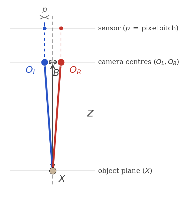
Fig. 17 Two camera centres \(O_L, O_R\) separated by baseline \(B\), viewing a specimen point \(X\) at working distance \(Z\). The pixel pitch \(p\) is shown on the left sensor.

The central pinhole stereo model is defined by the two intrinsic matrices and the stereo baseline or transform:

\[\mathcal M_{\mathrm{pinhole}} = \left(K_L,K_R,T_{R\leftarrow L}\right).\]

For channel c, let

\[(x_c,y_c)=\pi_{K_c}^{-1}(u_c,v_c).\]

The channel-frame direction is

\[d_{0,c}(u_c,v_c)= \frac{(x_c,y_c,1)^T}{\sqrt{x_c^2+y_c^2+1}}.\]

The left and right rays are

\[\mathcal R_L(u_L,v_L)=\left(0,d_{0,L}(u_L,v_L)\right),\]

\[\mathcal R_R^R(u_R,v_R)=\left(0,d_{0,R}(u_R,v_R)\right),\]

with the right ray transformed to the left frame using T_{L\leftarrow R} when triangulating. The physical-model-selection parameter vector is empty:

\[\theta_{\mathrm{pinhole}}=\varnothing.\]

The focal lengths and principal points are not absent; they are the fixed entries of K_L and K_R. The baseline is the fixed norm B=\|t_{R\leftarrow L}\|.

Candidate 1: central Brown-Conrady stereo

The Brown-Conrady stereo model adds per-channel distortion parameters to the central pinhole stereo geometry:

\[\mathcal M_{\mathrm{Brown}}= \left( K_L,K_R,T_{R\leftarrow L}, \theta_{\mathrm{Brown},L}, \theta_{\mathrm{Brown},R} \right),\]

with

\[\theta_{\mathrm{Brown},c}= (k_{1,c},k_{2,c},p_{1,c},p_{2,c},k_{3,c}).\]

The focal lengths, principal points and baseline remain the fixed K_L,K_R,T_{R\leftarrow L} values. For channel c, (x_{d,c},y_{d,c})=\pi_{K_c}^{-1}(u_c,v_c) are interpreted as distorted normalized coordinates. The undistorted coordinates (x_c,y_c) satisfy

\[x_{d,c} = x_c\left(1+k_{1,c}r_c^2+k_{2,c}r_c^4+k_{3,c}r_c^6\right) +2p_{1,c}x_cy_c+p_{2,c}(r_c^2+2x_c^2),\]

\[y_{d,c} = y_c\left(1+k_{1,c}r_c^2+k_{2,c}r_c^4+k_{3,c}r_c^6\right) +p_{1,c}(r_c^2+2y_c^2)+2p_{2,c}x_cy_c,\]

where r_c^2=x_c^2+y_c^2. The channel ray remains central:

\[\mathcal R_c(u_c,v_c)= \left( 0, \frac{(x_c,y_c,1)^T}{\sqrt{x_c^2+y_c^2+1}} \right).\]

Brown-Conrady can bend the direction field, but it cannot create a pixel-dependent origin field. It is therefore a useful misspecification test on non-central optics.

Candidate 2: pinhole stereo plus inclined parallel plates

The inclined-plate stereo model keeps the same stereo intrinsics and baseline, but places a plate in front of each channel:

\[\mathcal M_{\mathrm{plate}}= \left( K_L,K_R,T_{R\leftarrow L}, \theta_{\mathrm{plate},L}, \theta_{\mathrm{plate},R}, \eta_L,\eta_R,d_{1,L},d_{1,R} \right).\]

The fitted per-channel parameters are

\[\theta_{\mathrm{plate},c}=(\alpha_c,\beta_c,e_c).\]

The refractive index \eta_c and the first-interface distance d_{1,c} are fixed by default. For channel c, the pinhole direction before the plate is

\[s_c(u_c,v_c)= \frac{(x_c,y_c,1)^T}{\sqrt{x_c^2+y_c^2+1}}, \qquad (x_c,y_c)=\pi_{K_c}^{-1}(u_c,v_c).\]

The plate normal is

\[q_c(\alpha_c,\beta_c)= \frac{(\tan\alpha_c,\tan\beta_c,1)^T} {\sqrt{\tan^2\alpha_c+\tan^2\beta_c+1}}.\]

Define

\[c_c=q_c\cdot s_c, \qquad s_{\perp,c}=s_c-c_cq_c, \qquad \beta_{g,c}=\sqrt{1-\frac{\|s_{\perp,c}\|^2}{\eta_c^2}}.\]

The direction inside the plate, entry point, and exit point are

\[s_{g,c}=\frac{s_{\perp,c}}{\eta_c}+\beta_{g,c}q_c, \qquad I_{1,c}=\frac{d_{1,c}}{q_c\cdot s_c}s_c, \qquad I_{2,c}=I_{1,c}+\frac{e_c}{\beta_{g,c}}s_{g,c}.\]

The channel ray is

\[\mathcal R_{\mathrm{plate},c}(u_c,v_c)= \left(I_{2,c}(u_c,v_c),s_c(u_c,v_c)\right).\]

The exit point I_{2,c} is not set to zero. Changing d_{1,c} moves I_{2,c} along the emergent line and is therefore a longitudinal gauge for a parallel plate; this is why d_{1,c} is fixed in the default fit. The baseline still comes from T_{R\leftarrow L} and is not replaced by the plate thickness.

Candidate 3: non-central polynomial surrogate channels

The non-central polynomial surrogate uses effective per-channel origins rather than a shared physical CMO rig. The fixed and fitted quantities are:

\[\mathcal M_{\mathrm{CMO}}= \left( K_L,K_R, R_L,R_R, O_L,O_R, \theta_{\mathrm{dist},L},\theta_{\mathrm{dist},R}, \theta_{\mathrm{aberr},L},\theta_{\mathrm{aberr},R} \right).\]

For channel c, the intrinsic matrix is

\[\begin{split}K_c= \begin{pmatrix} f_{x,c} & 0 & c_{x,c}\\ 0 & f_{y,c} & c_{y,c}\\ 0 & 0 & 1 \end{pmatrix}.\end{split}\]

The effective CMO stereo baseline is the distance between fitted sub-pupil origins:

\[B_{\mathrm{CMO}}=\|O_R-O_L\|.\]

In the current independent channel fit, each channel estimates its own effective origin

\[O_c=(O_{x,c},O_{y,c},0)^T,\]

so the reported stereo CMO baseline is reconstructed afterwards from the left and right fitted origins. The current fittable candidate keeps K_c, image size (W,H) and channel orientation R_c fixed, and fits

\[\theta_{\mathrm{CMO},c}= \left[ O_{x,c},O_{y,c}, k_{1,c},k_{2,c},p_{1,c},p_{2,c},k_{3,c}, a^x_{1,c},\ldots,a^x_{m,c}, a^y_{1,c},\ldots,a^y_{m,c} \right].\]

The pixel-to-direction pipeline is

\[(x_{d,c},y_{d,c})=\pi_{K_c}^{-1}(u_c,v_c),\]

\[(x_c,y_c)=D_{\mathrm{Brown}}^{-1} (x_{d,c},y_{d,c}; k_{1,c},k_{2,c},p_{1,c},p_{2,c},k_{3,c}),\]

\[\Delta x_c(x_c,y_c)= \sum_{\ell=1}^{m} a^x_{\ell,c}\phi_\ell(x_c,y_c), \qquad \Delta y_c(x_c,y_c)= \sum_{\ell=1}^{m} a^y_{\ell,c}\phi_\ell(x_c,y_c).\]

The channel-frame direction is

\[d_{\mathrm{cam},c}(u_c,v_c)= \frac{(x_c+\Delta x_c,\;y_c+\Delta y_c,\;1)^T} {\sqrt{(x_c+\Delta x_c)^2+(y_c+\Delta y_c)^2+1}}.\]

The output ray is

\[\mathcal R_{\mathrm{CMO},c}(u_c,v_c)= \left( O_c, R_c\,d_{\mathrm{cam},c}(u_c,v_c) \right).\]

In the synthetic CMO generator there can also be a common aberration \theta_{\mathrm{common}} and differential channel aberrations \theta_{\mathrm{diff},L},\theta_{\mathrm{diff},R}:

\[\theta_{\mathrm{aberr},c} = \theta_{\mathrm{common}}+\theta_{\mathrm{diff},c}.\]

The current model-selection candidate fits only this effective per-channel sum. It does not yet decompose common and differential aberrations in a shared stereo fit. The rendered CMO generator and the fittable CMO candidate use the same intrinsics, Brown-Conrady, sub-pupil-origin, and polynomial ray-aberration primitives from stereocomplex.physics, so generation and fitting do not maintain two separate implementations of the optical model.

This candidate should be read as a generic non-central surrogate. It is useful when a true common-main-objective constraint would be too strong: independent objective microscopes, unknown stereo microscopes, asymmetric relay optics, tilted sensors, or channel-specific windows can all create smooth rayfields that are not representable by the physical CMO model below.

Candidate 4: physical CMO stereo model

The physical CMO model is a shared-rig stereo candidate:

\[\mathcal M_{\mathrm{CMO,phys}} = \left( f_{\mathrm{obj}}, Z_w, b, f_{\mathrm{tube}}, c_x,c_y, \theta_y, \theta_{\mathcal D,L}, \theta_{\mathcal D,R}; p\ \mathrm{fixed} \right).\]

It is defined in detail in Physical CMO Model. The main difference from the polynomial surrogate is structural: the two channels share the same main-objective geometry, their effective sub-pupils are separated by the baseline b, and their chief rays converge to the working plane Z_w.

For channel c, with s_L=-1 and s_R=+1, the effective sub-pupil is

\[S_c = \left( s_c\frac{b}{2}, 0, Z_w-f_{\mathrm{obj}} \right)^T,\]

and the pixel-selected point on the working plane is

\[P_c(u,v)= \left( Z_w\alpha_x, Z_w\alpha_y, Z_w \right)^T,\]

where (\alpha_x,\alpha_y) are angular coordinates obtained from fixed pixel pitch, tube focal length and effective Brown-Conrady-like direction undistortion. The CMO ray is

\[\mathcal R_c(u,v)= \left( S_c, \frac{P_c(u,v)-S_c}{\|P_c(u,v)-S_c\|} \right).\]

From ray geometry alone, f_tube and pixel pitch are identifiable through their ratio p/f_tube, not separately. StereoComplex therefore fixes pixel_pitch_mm from sensor metadata and optimizes f_tube_mm. The physical CMO reference page reports this as an identifiability limit rather than hiding it in the optimizer.

The default shared-principal-point mode has 17 fitted parameters. An aligned sensor mode adds two centered principal-point offset degrees of freedom, (\Delta c_x,\Delta c_y), and has 19 fitted parameters. This mode is useful for real microscopes where the two sensors are not mechanically aligned to the same principal point; horizontal offset can still correlate with the fitted sub-pupil baseline, so the ray-space residual is the primary validation.

Scientific background for the polynomial surrogate

The polynomial channel model is an effective ray-space model, not a full lens-design model. Its purpose is to provide a compact, identifiable parameterization for measured CMO-like rayfields. The model is built from standard pieces rather than from a single named closed-form microscope model:

Model block	Role in StereoComplex	Background
Common-main-objective stereo geometry	left/right effective sub-pupil origins and channel rays through a shared objective family	Nikon MicroscopyU describes CMO stereomicroscopes as designs where image-forming light enters a common main objective and is separated into two optical paths; its optical-path tutorial describes the two parallel bundles used by the channels.
Generic / non-central camera model	pixel \rightarrow 3D line, allowing a channel not to have one unique pinhole center	Grossberg and Nayar’s raxel model and the general-camera calibration papers by Sturm and by Ramalingam, Sturm and Lodha motivate ray-based calibration for arbitrary cameras.
Brown-Conrady distortion	central radial/tangential direction component per channel	Conrady’s decentering distortion model and Brown’s photogrammetric lens-distortion model are the classical sources for the radial/decentering distortion family used in calibration software.
Smooth polynomial ray aberration	low-order angular surrogate for residual optical aberration	Optical aberrations are commonly represented by low-order polynomial bases, especially Zernike-type bases on pupils; see Born and Wolf and Mahajan for standard optical-aberration background.

The implemented polynomial terms are therefore best interpreted as a low-order angular aberration surrogate in normalized ray coordinates. They are not a direct wavefront expansion, and their coefficients should not be read as unique lens-design parameters. In practice, the stable physical quantities are the ray-space residuals, effective sub-pupil origins, recovered stereo baseline, and pose consistency; individual Brown and polynomial coefficients can be correlated.

Useful references:

• M. D. Grossberg and S. K. Nayar, “The Raxel Imaging Model and Ray-Based Calibration,” International Journal of Computer Vision, 61(2), 119-137, 2005. PDF: https://www.cs.columbia.edu/CAVE/publications/pdfs/Grossberg_IJCV05.pdf

• P. Sturm, “Multi-view Geometry for General Camera Models,” CVPR, 2005.

• S. Ramalingam, P. Sturm and S. K. Lodha, “Towards Complete Generic Camera Calibration,” CVPR, 2005. PDF: https://perception.inrialpes.fr/Publications/2005/RSL05a/RamalingamSturmLodha-cvpr05.pdf

• A. E. Conrady, “Decentred Lens-Systems,” Monthly Notices of the Royal Astronomical Society, 79, 384-390, 1919.

• D. C. Brown, “Decentering Distortion of Lenses,” Photogrammetric Engineering, 32(3), 444-462, 1966.

• M. Born and E. Wolf, Principles of Optics, 7th expanded edition, Cambridge University Press, 1999.

• V. N. Mahajan, “Zernike Circle Polynomials and Optical Aberrations of Systems with Circular Pupils,” Applied Optics, 33(34), 8121-8124, 1994. DOI page: https://opg.optica.org/abstract.cfm?uri=ao-33-34-8121

• Nikon MicroscopyU, “Introduction to Stereomicroscopy” and “Stereomicroscope Optical Pathways” for technical background on Greenough and common-main-objective stereomicroscope layouts: https://www.microscopyu.com/techniques/stereomicroscopy/introduction-to-stereomicroscopy, https://www.microscopyu.com/tutorials/smzpaths.

Information criteria

For each candidate, let

\[RSS=\sum_i r_i^2,\]

where r_i are scalar residual components. Let N_s be the number of scalar residuals and N_p the number of sampled pixel/ray observations. For the two-plane residual, N_s = 6 N_p. StereoComplex reports

\[\mathrm{AIC}=2p+N_s\log\left(\frac{RSS}{N_s}\right),\]

\[\mathrm{BIC}=p\log(N_p)+N_s\log\left(\frac{RSS}{N_s}\right).\]

The likelihood term uses scalar metric residuals. The BIC complexity penalty uses sampled pixels as the independent observation count. This keeps the penalty tied to the number of independent rays while retaining the metric information from both reference planes.

Minimum example

from pathlib import Path
import stereocomplex as sc

board = sc.CharucoBoardSpec(
    squares_x=9,
    squares_y=6,
    square_size_mm=20.0,
    marker_size_mm=15.0,
    aruco_dictionary="DICT_4X4_50",
)

# Step 1: measure the rayfield from image folders.
fit = sc.fit_stereo_zernike_origin_field_from_image_dirs(
    left_dir=Path("my_data/left"),
    right_dir=Path("my_data/right"),
    board=board,
    max_order=4,
    method2d="rayfield_tps_robust",
)

# Step 2: identify the physical optics.
report = sc.select_physical_model_from_rayfield(
    target_field=fit.left_field,
    candidate_specs=None,          # default: pinhole, Brown-Conrady, inclined plate
    K=fit.left_field.K,
    image_size=fit.left_field.config.image_size,
)

print(report.best_by_bic)
for row in report.rows():
    print(row)

How to read the report

report.rows() returns a list of dicts with these keys:

Key	Description
model	Model name, for example central_pinhole, central_brown_conrady, pinhole_parallel_plate, or polynomial_surrogate_channel.
parameters	Number of free parameters fitted.
rms_mm	Primary unweighted RMS distance on the observed support, in mm. If no separate support is supplied, this is the full-grid RMS.
support_rms_mm	RMS on the observed pixel support only.
full_grid_rms_mm	RMS on a dense full-image grid (extrapolation quality).
bic	Bayesian Information Criterion (lower is better).
aic	Akaike Information Criterion (lower is better).
selected_bic	True for the BIC winner.

report.best_by_bic is a string name; report.best_by_rms and report.best_by_aic are available for alternative criteria.

Interpretation guide:

• A large gap in rms_mm between first and second candidate is a strong signal.

• support_rms_mm measures fit quality on observed pixels; full_grid_rms_mm measures extrapolation quality, which is more sensitive to model misspecification at the image edges.

• If BIC and AIC disagree, prefer BIC for compact models on typical calibration grids (BIC penalises free parameters more strongly).

Example result on the inclined-plate oracle

On the synthetic inclined-plate benchmark, the stereo-pair summary looks like:

model	parameters	rms_mm	support_rms_mm	full_grid_rms_mm	bic	selected_bic
central_pinhole	0	2.990	2.990	3.714	+1 052	False
central_brown_conrady	10	2.143	2.143	2.649	−10 772	False
pinhole_parallel_plate	6	0.000258	0.000258	0.00335	−306 399	True

The plate model wins by a factor of more than 8000× in support RMS relative to Brown-Conrady. This is expected: the oracle is an inclined plate, and the plate model has the right structural degrees of freedom.

Adding a custom candidate model

Implement the PhysicalRayFieldModel protocol — a class with a ray(u, v) method and optionally from_parameter_vector, parameter_dict, n_parameters. Then wrap it in a PhysicalModelSpec and pass a list as candidate_specs:

import numpy as np
from stereocomplex.physics import PhysicalModelSpec

class MyTiltModel:
    """A custom physical candidate: single-axis tilt only."""
    name = "my_tilt"

    def __init__(self, K, tilt_deg=0.0):
        self.K = K
        self.tilt_deg = tilt_deg

    @classmethod
    def from_parameter_vector(cls, x, K, **kwargs):
        return cls(K=K, tilt_deg=float(x[0]))

    def parameter_dict(self):
        return {"tilt_deg": float(self.tilt_deg)}

    def ray(self, u, v):
        # ... your ray computation here
        ...

my_spec = PhysicalModelSpec(
    name="my_tilt",
    model_class=MyTiltModel,
    initial_parameters=np.zeros(1),
    bounds=(np.array([-45.0]), np.array([45.0])),
)

report = sc.select_physical_model_from_rayfield(
    target_field=fit.left_field,
    candidate_specs=[my_spec],     # only test your model
    K=fit.left_field.K,
    image_size=fit.left_field.config.image_size,
)

Or extend the default set:

from stereocomplex.advanced import default_physical_model_specs

specs = default_physical_model_specs() + [my_spec]
report = sc.select_physical_model_from_rayfield(
    target_field=fit.left_field,
    candidate_specs=specs,
    K=K,
    image_size=image_size,
)

Pitfalls

BIC uses a mixed scalar/observation convention. See Information criteria for the exact convention: the fit likelihood uses scalar residual components, while the BIC penalty uses sampled pixels/rays as independent observations.

Support vs. extrapolation. By default, full_grid_weight=0.25 adds a dense evaluation grid weighted at 25 % of the support. The full_grid_rms_mm column measures how well each model extrapolates beyond the calibration grid; models with wrong structure (e.g., a central model on a non-central rig) often have larger extrapolation residuals than support residuals.

Convergence of the Brown-Conrady fitter. The undistortion loop uses 10 fixed-point iterations. For strongly distorted optics (|k1| > 0.5), convergence may be slow. Increase max_nfev or tighten bounds in the PhysicalModelSpec if needed.

A low RMS does not mean the model is “correct”. A plate model with 3 parameters can achieve near-zero residuals on a plate oracle because it has the right structure. But on a real rig with a complex non-central signature, all models may show residuals, and the BIC winner is simply the most compact viable explanation — not a ground-truth identification.