Worked example: raw OpenCV ChArUco vs a ray-field second pass (errors + plots)

Goal: given stereo image pairs (left/right), compare:

1. raw ChArUco corners obtained with standard OpenCV routines,

2. a second non-parametric pass (a planar ray-field: homography + smoothed residual field),

3. the 2D error in pixels against ground truth (when available, typically in synthetic data),

4. diagnostic plots (ECDF + histograms).

This example is designed to be reproducible end-to-end by a Master’s-level student.

Prerequisites

• Python + numpy

• opencv-contrib-python (required for cv2.aruco)

Plot generation does not rely on matplotlib: plots are rendered directly with OpenCV to minimize dependencies.

Expected data

The script runs out of the box on the repository dataset v0 format (see docs/DATASET_SPEC.md):

dataset/v0_png/train/scene_0000/
  meta.json
  frames.jsonl
  left/000000.png
  right/000000.png
  gt_charuco_corners.npz

True error (against GT) requires gt_charuco_corners.npz (therefore typically synthetic data).

Theory recap: a planar ray-field (a non-parametric warp on the board plane)

Notation:

• \((x,y)\): coordinates on the board plane (mm),

• \(\mathbf{u}(x,y)=(u(x,y),v(x,y))^\top\): image coordinates (px),

• \(\tilde{\mathbf{x}}=(x,y,1)^\top\): homogeneous coordinates.

Define the projection operator (homogeneous → inhomogeneous):

(1)\[\begin{split}\pi\!\left(\begin{bmatrix}a\\b\\c\end{bmatrix}\right)=\begin{bmatrix}a/c\\b/c\end{bmatrix}.\end{split}\]

The key idea is not to impose a pinhole model \((K,\mathbf d)\), but to exploit:

• the “planar target” structure,

• a low-frequency prior on the plane→image mapping.

We write the mapping as:

(2)\[\mathbf{u}(x,y) = \pi(H\tilde{\mathbf{x}}) + \mathbf{r}(x,y)\]

• \(H\): global homography (projective backbone),

• \(\mathbf{r}(x,y)\): a smoothed 2D residual field learned from ArUco markers.

Terminology (“non-parametric”):

• Here, “non-parametric” does not mean “parameter-free”: we do estimate parameters.

• It means “no low-dimensional optical model” (no pinhole + distortion \((K,\mathbf d)\)); instead we estimate a smooth regression of a 2D warp over the plane, with complexity controlled by grid resolution and regularization.

• More strictly, this is semi-parametric: a parametric projective base (\(H\)) + a smooth correction (\(\mathbf r\)).

Why a homography is a good base (planar board)

Without distortion, a pinhole camera observes a planar target through a homography. If the board lies in the plane \(Z=0\) of the board frame, and the camera has pose \((R,t)\) and intrinsic matrix \(K\), then:

(3)\[s\,\tilde{\mathbf{u}} \;=\; K \,[\,\mathbf r_1\;\mathbf r_2\;\mathbf t\,]\;\tilde{\mathbf{x}} \quad\Rightarrow\quad \tilde{\mathbf{u}} \sim H\,\tilde{\mathbf{x}}, \;\; H = K [\,\mathbf r_1\;\mathbf r_2\;\mathbf t\,].\]

where \(\tilde{\mathbf{u}}=(u,v,1)^\top\) and \(\mathbf r_1,\mathbf r_2\) are the first two columns of \(R\). This justifies \(\pi(H\tilde{\mathbf x})\) as a good global approximation (perspective + pose) of the board→image mapping.

Distortion/aberrations: what a homography cannot explain

In this repository, synthetic images typically include Brown distortion (radial + tangential). More generally, distortion can be seen as a smooth mapping \(d(\cdot)\) acting on ideal image coordinates:

(4)\[\mathbf u(x,y) \;=\; d\!\left(\pi(H\tilde{\mathbf x})\right).\]

If we write \(d(\mathbf u)=\mathbf u + \Delta(\mathbf u)\) (with \(\Delta\) the distortion offset), then:

(5)\[\mathbf u(x,y) \;=\; \pi(H\tilde{\mathbf x}) + \underbrace{\Delta\!\left(\pi(H\tilde{\mathbf x})\right)}_{\mathbf r(x,y)}.\]

In real optics (and in simulators), \(\Delta\) is typically low-frequency (radial polynomials, decentering, etc.), hence \(\mathbf r(x,y)\) is smooth on the board plane. The homography captures the dominant projective geometry, and \(\mathbf r\) captures a non-parametric correction of aberrations (at least their smooth component on the plane).

Estimation objective (data term + regularization)

Given ArUco correspondences \(\{(x_i,y_i)\leftrightarrow \mathbf{u}_i\}_{i=1}^N\), we:

1. estimate a robust homography \(H\) (RANSAC),

2. compute observed residuals \(\hat{\mathbf r}_i\),

3. reconstruct a smooth field \(\mathbf r_\theta(x,y)\) that approximates these residuals.

We parameterize \(\mathbf r(x,y)\) by values on a regular grid in board coordinates.

Definition of \(\theta\) (field parameters):

• Choose a grid of \(M\) nodes at positions \(\{(x_m,y_m)\}_{m=1}^M\).

• Associate to each node an unknown 2D residual \(\mathbf g_m=(g^x_m,g^y_m)^\top\) (pixels, horizontal/vertical components).

• Stack them into a parameter vector \(\theta\) (minimizing with respect to \(\theta\) is exactly minimizing with respect to all \(\mathbf g_m\)):

(6)\[\theta=\begin{bmatrix} g^x_1&\cdots&g^x_M&g^y_1&\cdots&g^y_M \end{bmatrix}^\top \in\mathbb{R}^{2M}.\]

Field evaluation (bilinear interpolation): for a point \((x,y)\), take the 4 nodes of the cell containing \((x,y)\) and bilinear weights \(\{w_m(x,y)\}\) (sum to 1), yielding:

(7)\[\begin{split}\mathbf r_\theta(x,y) =\sum_{m=1}^{M} w_m(x,y)\,\mathbf g_m =\begin{bmatrix} \sum_m w_m(x,y)\,g^x_m\\ \sum_m w_m(x,y)\,g^y_m \end{bmatrix}.\end{split}\]

We then solve:

(8)\[\min_{\theta}\sum_{i=1}^N \rho\!\left(\left\|\mathbf r_\theta(x_i,y_i)-\hat{\mathbf r}_i\right\|_2^2\right) + \lambda \|L\theta\|_2^2\]

• \(L\): discrete Laplacian on the grid (penalizes curvature, enforces smoothness),

• \(\lambda\): regularization weight,

• \(\rho(\cdot)\): robust loss (Huber) to limit the influence of outliers.

The (norm-based) Huber loss can be written as:

(9)\[\begin{split}\rho(t)= \begin{cases} t, & \sqrt{t}\le \delta,\\ 2\delta \sqrt{t} - \delta^2, & \sqrt{t}>\delta, \end{cases}\end{split}\]

and is efficiently solved by IRLS (iteratively reweighted least squares). Weights are \(w_i=1\) if \(\lVert\cdot\rVert\le\delta\) and \(w_i=\delta/\lVert\cdot\rVert\) otherwise.

Available measurements (ArUco)

Each detected ArUco corner provides a noisy correspondence:

(10)\[\mathbf{u}_i \approx \mathbf{u}(x_i,y_i)\]

We first estimate \(H\) via RANSAC, then compute observed residuals:

(11)\[\hat{\mathbf r}_i = \mathbf{u}_i - \pi(H\tilde{\mathbf{x}}_i)\]

Why this can reduce uncertainty without an optical model

Model a measurement as:

(12)\[\mathbf{u}_i = \mathbf{u}(x_i,y_i) + \boldsymbol\varepsilon_i\]

where \(\boldsymbol\varepsilon_i\) includes detection noise, bias (blur/compression), and outliers.

The key point is that \(\mathbf r(x,y)\) is estimated using all available ArUco measurements under a smoothness prior:

• if aberrations (more generally, deviations from the projective model) are dominated by a smooth component on the plane, then \(\mathbf r\) captures a systematic correction (bias) that a homography alone cannot explain;

• if detection noise is locally uncorrelated, smoothing acts as denoising (variance reduction) by enforcing spatial coherence.

This is a bias/variance trade-off:

• too much smoothing \(\Rightarrow\) bias (real variations are flattened),

• too little smoothing \(\Rightarrow\) variance (the model follows noise/outliers).

In practice, Brown distortion and many “non-ideal optics” effects are smooth enough that \(\mathbf r\) reduces error over the whole board, including on ChArUco corners not directly used to fit \(\mathbf r\).

Why not “just Gaussian blur the residuals”?

Applying a Gaussian filter to suppress high frequencies makes sense if one already has a dense residual field defined on a regular grid.

Here, residuals \(\hat{\mathbf r}_i\) are observed only at a limited number of points (Aruco corners), with:

• irregular sampling (marker geometry),

• large unobserved regions (between markers / borders / masks),

• outliers (failed detections, compression, blur, etc.).

Therefore, before “blurring”, one must solve an interpolation/inpainting problem from sparse samples. The \(\mathbf r_\theta\) (grid + interpolation) model with \(\|L\theta\|^2\) regularization provides:

• an explicit grid representation,

• controlled smoothness (Laplacian / Tikhonov regularization),

• robustness to outliers (Huber/IRLS), which a plain Gaussian blur does not provide.

In other words, Gaussian blur is an option after reconstructing a dense field; the method here integrates (1) reconstruction + (2) smoothing + (3) robustness in one estimator.

TPS variant (thin-plate splines) for residual reconstruction

A classical alternative to the bilinear grid is a regularized TPS (thin-plate spline), well-suited to sparse measurements.

After fitting the base homography, we observe residuals \(\hat{\mathbf r}_i\) at ArUco points \((x_i,y_i)\) and fit two scalar TPS (for \(r^x\) and \(r^y\)):

(13)\[r(x,y)=a_0+a_1 x+a_2 y+\sum_{i=1}^{N} w_i\,U(\lVert (x,y)-(x_i,y_i)\rVert), \qquad U(r)=r^2\log(r^2)\;\; (U(0)=0).\]

In practice, coefficients \(\{w_i\}\) and \(\{a_k\}\) are found by solving a linear system:

(14)\[\begin{split}\begin{bmatrix} K+\lambda I & P\\ P^\top & 0 \end{bmatrix} \begin{bmatrix} w\\ a \end{bmatrix} = \begin{bmatrix} \hat r\\ 0 \end{bmatrix},\end{split}\]

where \(K_{ij}=U(\lVert \mathbf x_i-\mathbf x_j\rVert)\), \(P=[\mathbf 1,\;x,\;y]\), and \(\lambda\) controls smoothness (larger \(\lambda\) makes the field more “rigid”).

In this repository, the variant is available via rayfield_tps (homography + TPS on residuals). On dataset/v0_png/train/scene_0000, with the current default (tps_lam≈10), it is slightly better than the grid backend:

• left RMS: ~0.219 px (rayfield_tps) vs ~0.224 px (rayfield)

• right RMS: ~0.153 px (rayfield_tps) vs ~0.161 px (rayfield)

What this corrects (and what it does not)

This model typically improves:

• smooth geometric distortions (radial/tangential) and, more generally, any low-frequency deviation of the plane→image mapping,

• part of localization biases induced by blur/compression, as long as they appear as a spatially coherent offset.

It does not “fix”:

• high-frequency errors (aliasing, localized artifacts, occlusions),

• out-of-plane effects (if the board is not planar, the assumption breaks),

• a physically grounded 3D ray model (this remains a 2D warp on the plane).

Important notes (what this “ray-field” is not)

• This is a 2D warp restricted to the board plane: it does not reconstruct a per-pixel 3D ray field \((\mathbf{o}(u,v),\mathbf{d}(u,v))\).

• It is designed as a 2D stabilization second pass when a pinhole model (PnP) is inadequate (e.g., non-central/CMO systems).

Pipeline: what the example actually does

For each left and right image:

1. Build a CharucoBoard from meta.json (square size, marker size, ArUco dictionary).

2. Detect ArUco markers (IDs + 4 detected 2D corners per marker).

3. Extract raw ChArUco corners via OpenCV (interpolation from detected markers).

4. Estimate a homography \(H\) between board-space ArUco corners and image-space corners.

5. Compute residuals \(\hat{\mathbf r}_i\), then fit a smoothed residual field \(\mathbf r(x,y)\) (grid + IRLS/Huber or TPS).

6. Predict all ChArUco corners via \(\pi(H\tilde{\mathbf{x}}) + \mathbf r(x,y)\).

7. Compare to GT corners (if available) and produce:

   • a summary (RMS, P50, P95),

   • ECDF + histogram plots,

   • visual overlays (optional).

Where is the code?

• Runnable script: docs/examples/rayfield_charuco_end_to_end.py

• Ray-field implementation (used by the script): src/stereocomplex/eval/charuco_detection.py (_predict_points_rayfield_tps_robust)

Coordinate convention (important)

In this repository, GT uses the “pixel centers at integer coordinates” convention.

In the current implementation (and in the script):

• OpenCV ChArUco corners are corrected by -0.5 px (typical OpenCV shift),

• AruCo corners used for homography/ray-field are not corrected (already consistent).

Running the example

Command (on the reference dataset used in this repo):

.venv/bin/python docs/examples/rayfield_charuco_end_to_end.py dataset/v0_png \
  --split train --scene scene_0000 \
  --out docs/assets/rayfield_worked_example \
  --save-overlays

By default, the example uses the current recommended variant: rayfield_tps_robust (homography + TPS residual + IRLS/Huber) with tps_lam=10. To use the historical “bilinear grid + Laplacian + Huber/IRLS” backend:

.venv/bin/python docs/examples/rayfield_charuco_end_to_end.py dataset/v0_png \
  --split train --scene scene_0000 \
  --out docs/assets/rayfield_worked_example \
  --save-overlays \
  --rayfield-backend grid

Outputs:

• docs/assets/rayfield_worked_example/summary.json: per-view metrics,

• docs/assets/rayfield_worked_example/plots/ecdf_left.png, ecdf_right.png,

• docs/assets/rayfield_worked_example/plots/hist_left.png, hist_right.png,

• docs/assets/rayfield_worked_example/overlays/left_frame000000.png, right_frame000000.png (if --save-overlays).

Plots (examples)

These figures are generated automatically by the command above.

ECDF (cumulative distribution of error)

See Fig. 2 and Fig. 3.

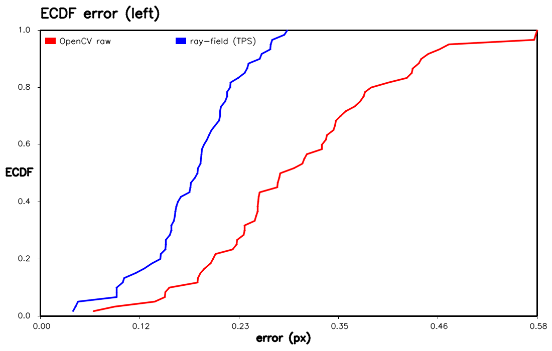
Fig. 2 2D error ECDF (left view): raw OpenCV vs ray-field second pass (TPS).

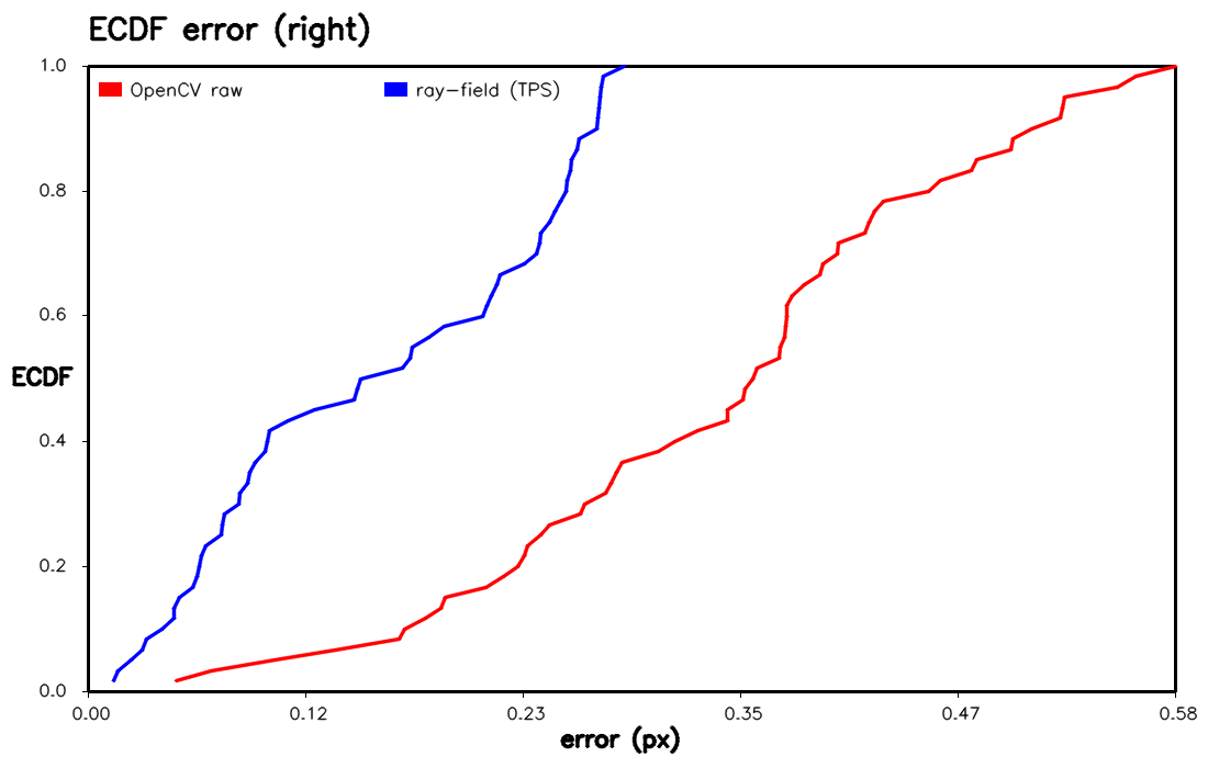
Fig. 3 2D error ECDF (right view): raw OpenCV vs ray-field second pass (TPS).

Histograms

See Fig. 4 and Fig. 5.

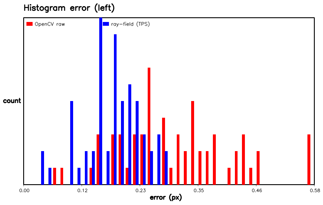
Fig. 4 2D error histogram (left view).

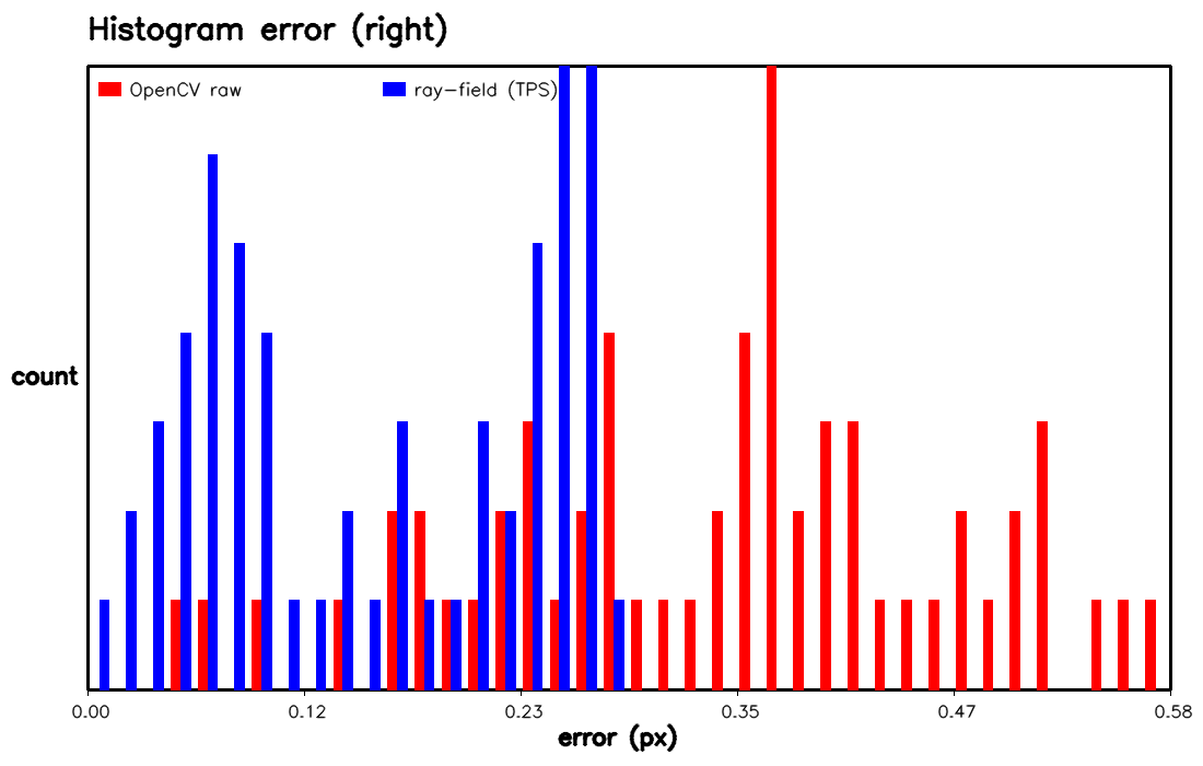
Fig. 5 2D error histogram (right view).

Sensitivity to \(\lambda\) (TPS)

Parameter tps_lam controls the smoothness/fit trade-off: small \(\lambda\) fits data more closely (risk of overfitting noise), large \(\lambda\) makes the field more rigid (risk of underfitting).

RMS and P95 vs \(\lambda\) (on the example scene):

See Fig. 6 and Fig. 7.

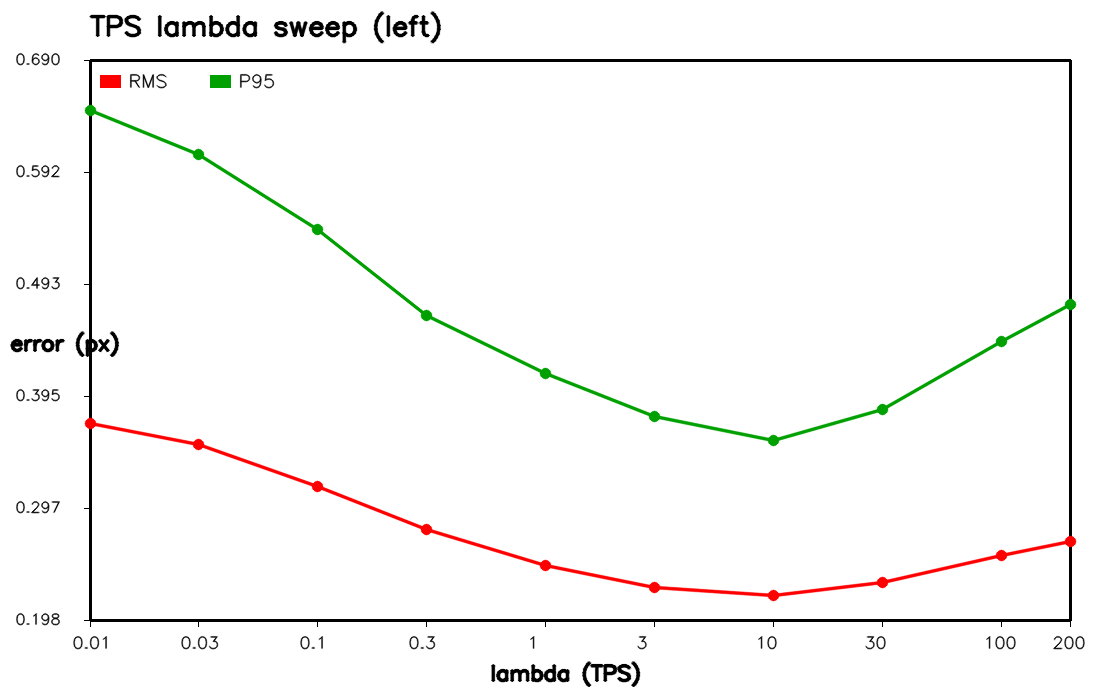
Fig. 6 TPS \(\lambda\) sensitivity: RMS and P95 vs tps_lam (left view).

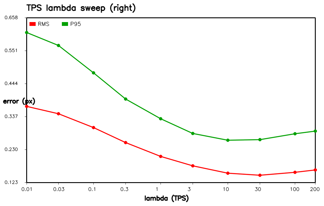
Fig. 7 TPS \(\lambda\) sensitivity: RMS and P95 vs tps_lam (right view).

Why different optima for left/right?

• The two cameras have different aberrations and noise (distortion + blur + ArUco detection), hence the overfit/underfit trade-off differs.

• The number and geometry of successfully detected markers can vary slightly between views, thus constraining the residual field differently.

Which \(\lambda\) should be used?

• In practice, one chooses a single \(\lambda\) for the system; a robust choice is a plateau close to the minima of both curves.

• On this scene, tps_lam=10 is close to the left minimum and very close to the right minimum; this is the default of the worked example.

Visualizing aberrations (residual amplitude)

We visualize the amplitude of the learned residual field on the plane, \(\lVert \mathbf r(x,y)\rVert\) (pixels), which highlights the low-frequency structure of the projected aberrations:

See Fig. 8 and Fig. 9.

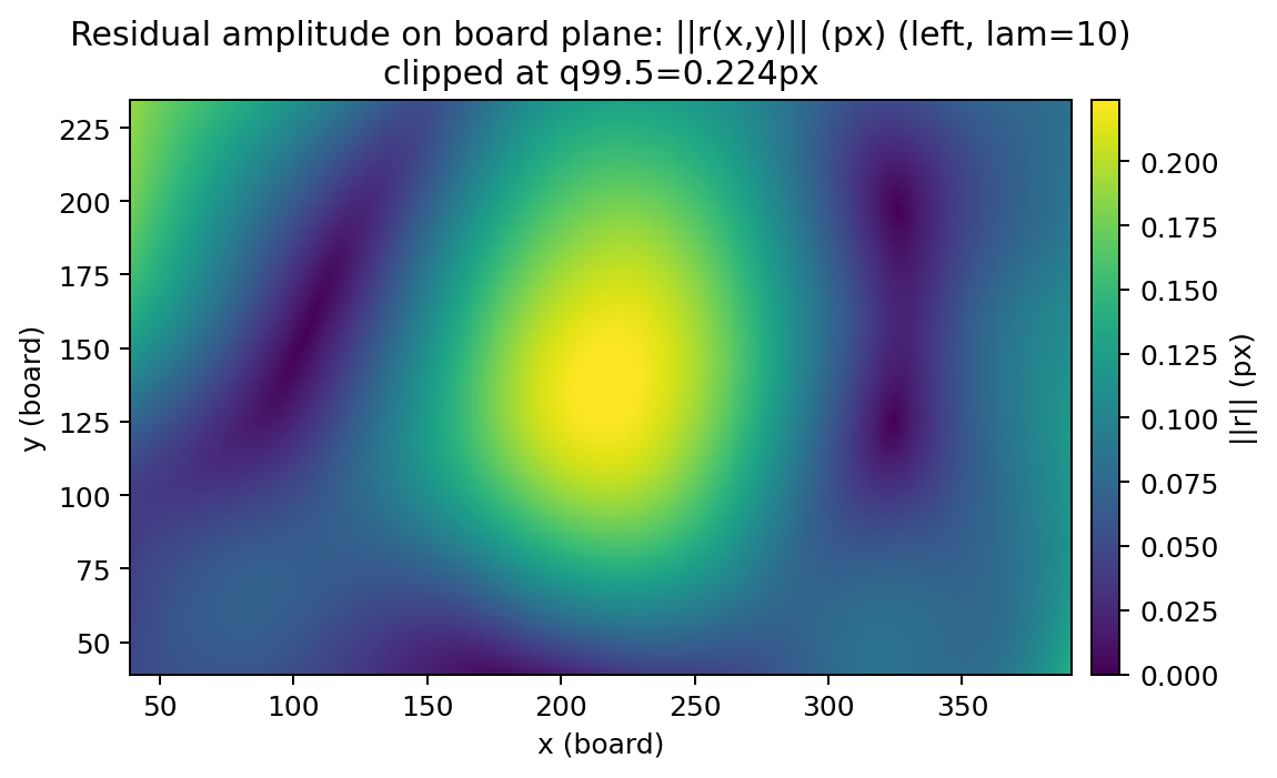
Fig. 8 Residual amplitude \(\lVert \mathbf r(x,y)\rVert\) (px) on the board plane (left view, frame 0).

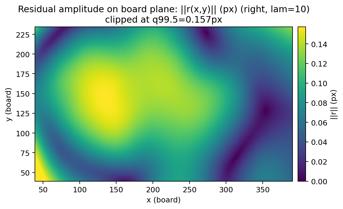
Fig. 9 Residual amplitude \(\lVert \mathbf r(x,y)\rVert\) (px) on the board plane (right view, frame 0).

Overlays (visual sanity checks)

See Fig. 10 and Fig. 11.

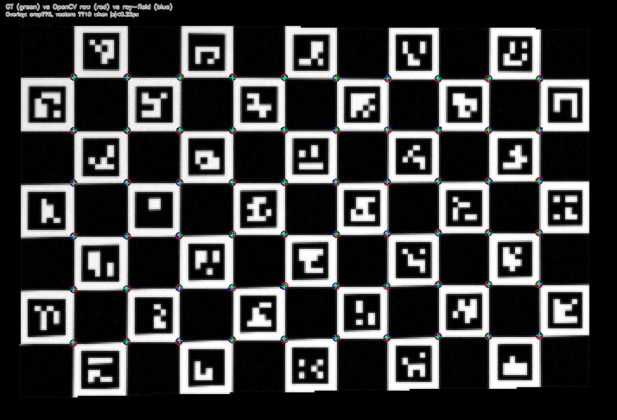
Fig. 10 Overlay (left view, frame 0): GT (green), raw OpenCV (red), ray-field (blue).

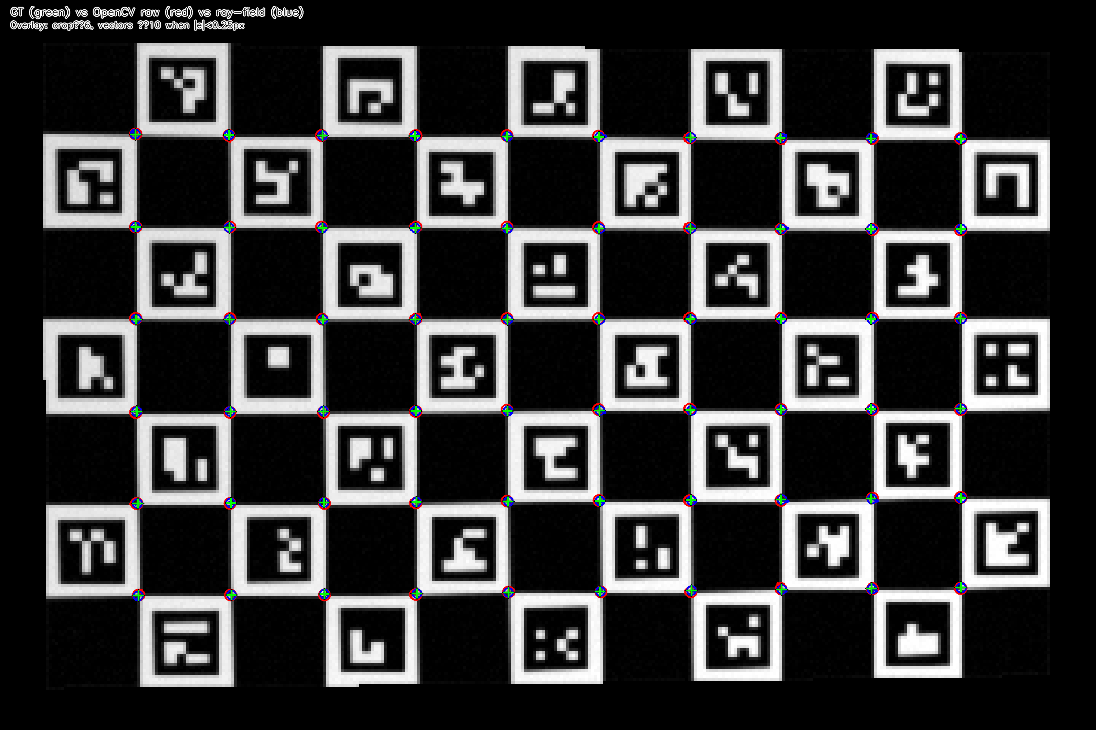
Fig. 11 Overlay (right view, frame 0): GT (green), raw OpenCV (red), ray-field (blue).

Ideal vs realistic (why GT may look “off”)

If the image includes blur / MTF / noise, the photometric corner (what your eye sees as the edge intersection) can be slightly shifted relative to the geometric GT (analytical projection). Here, GT includes the dataset’s geometric distortion (Brown model): the “ideal” vs “realistic” comparison does not remove distortion. For readability, the “ideal” image in Fig. 12 is a strict render: no blur/noise, and nearest-neighbor texture sampling (to avoid introducing an implicit MTF from texture resampling).

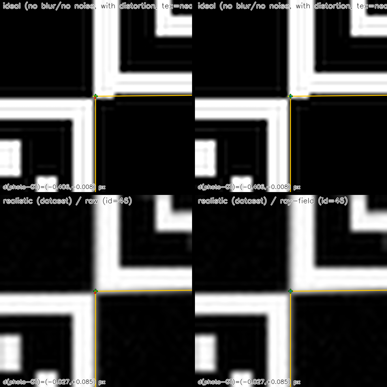
Fig. 12 2×2: ideal (top) vs realistic (bottom), raw (left) vs ray-field (right). GT is shown in green, predictions in red/blue, and the estimated “photometric corner” is shown as a yellow dot. Orange segments show the projected edges of a neighboring board square (geometry sanity-check): if these edges match the nearest-neighbor steps in the strict-ideal render, the projection (pose + distortion + conventions) is consistent and the remaining sub-pixel offset is photometric.

Photometric bias at checkerboard corners

In the overlays above, we deliberately distinguish geometric ground truth from what we call the photometric corner.

Geometric corner (ground truth). The geometric corner is defined as the intersection of two edges in the 3D model of the ChArUco board, projected into the image using the known pose and distortion model. It is a purely geometric quantity: it does not depend on image sampling, blur, noise, or the choice of corner detector. In the figures, it is shown as the green cross.

Photometric corner. The photometric corner is defined as the location in the sampled image that maximizes a photometric criterion (e.g., local edge-intersection estimate, corner response, gradient-based criterion). This is the quantity implicitly targeted by corner detectors and sub-pixel refinement algorithms. In the figures, it is shown as the yellow marker.

Photometric bias. We define the photometric bias as the vector difference between the photometric corner and the geometric corner (in image pixels):

\[\mathbf{b}_{\mathrm{photo}} = \mathbf{x}_{\mathrm{photo}} - \mathbf{x}_{\mathrm{geom}}.\]

This bias is not an error in the geometric projection model. It arises from the fact that the photometric corner is extracted from a discretely sampled intensity image, while the geometric corner is defined in continuous space.

Even in strict “ideal” renders (no blur/no noise, nearest-neighbor texture sampling), a non-zero photometric bias can appear due to:

• Rasterization effects (sharp edges discretized on a pixel grid).

• Local intensity structure near ArUco markers (the neighborhood is not a perfectly symmetric black–white “L” corner).

• Distortion and perspective (local anisotropy and edge orientation modify the sampled gradient field).

• Any implicit MTF introduced by rendering/resampling steps.

Key observation. In Fig. 12, the projected square edges (orange) coincide with the observed intensity transitions in the strict-ideal render, supporting that the geometric projection is consistent. The remaining offset between the green cross and the yellow marker is therefore photometric.

Micro-overlays (sub-pixel readability)

Two panels (left: raw, right: ray-field) on a few-pixel neighborhood (pixel grid displayed):

See Fig. 13 and Fig. 14.

Important: these micro-overlays show the pixel lattice (each big square is one source pixel, upscaled with nearest-neighbor). The GT cross is a sub-pixel location in a pixel-center coordinate system, so it is not expected to sit exactly on the grid-line intersections. Use the larger overlays above if you want to visually check the checkerboard geometry.

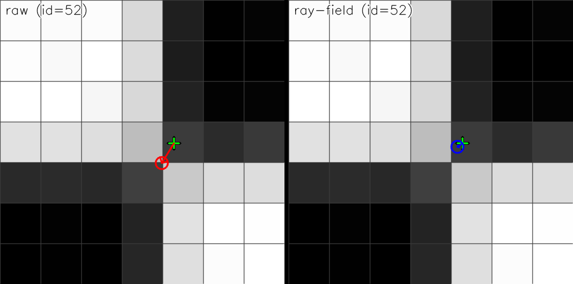
Fig. 13 Micro-overlay (left view, frame 0): example corner where the correction helps significantly (raw vs ray-field panels).

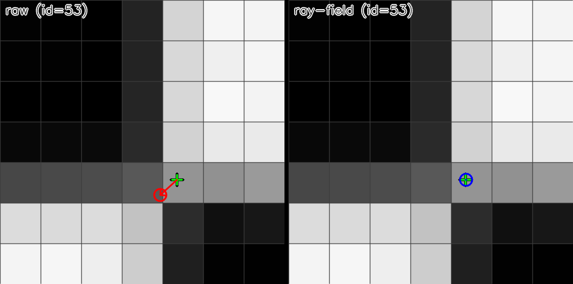
Fig. 14 Micro-overlay (right view, frame 0): example corner where the correction helps significantly (raw vs ray-field panels).

Board corner (±1 px neighborhood):

See Fig. 15 and Fig. 16.

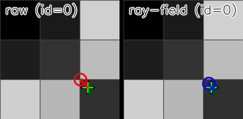
Fig. 15 Micro-overlay (left view, frame 0): board corner (±1 px neighborhood).

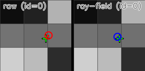
Fig. 16 Micro-overlay (right view, frame 0): board corner (±1 px neighborhood).

Overlay notes:

• Errors are often sub-pixel, so overlays are cropped around the board and then upscaled (--overlay-scale).

• Vectors represent GT→prediction residuals. When too small to be visible, vectors are amplified only for visualization (--overlay-min-vector-len, --overlay-vector-scale).

• Micro-overlays are controlled with --micro-radius (default 3 px), --micro-corner-radius (default 1 px) and --micro-scale (default 80×).

How to interpret results

• If ray-field is better, the ECDF should be shifted to the left (more small errors) and P95 should decrease.

• If smoothing is too strong (e.g. --smooth-lambda), one may smooth “real” variations → local bias (drift).

• If the dataset contains detection outliers (misdetected markers), increasing --huber-c or --iters can stabilize.

Extensions (suggested exercises)

• Sweep grid_size / smooth_lambda and plot RMS vs regularization.

• Compare homography (baseline) vs ray-field to isolate the contribution of the residual field.

• Test on multiple scenes/poses and study the effect of out-of-convex-hull regions (extrapolation).

References (bibliography pointers)

Classical references relevant to the approach (robust + regularized + smooth field from sparse correspondences):

• P. J. Huber, “Robust Estimation of a Location Parameter”, Annals of Mathematical Statistics, 1964. (Huber loss, IRLS)

• A. N. Tikhonov, V. Y. Arsenin, Solutions of Ill-posed Problems, 1977. (regularization, quadratic penalties)

• F. L. Bookstein, “Principal Warps: Thin-Plate Splines and the Decomposition of Deformations”, IEEE TPAMI, 1989. (smooth interpolation of 2D deformations)

• G. Wahba, Spline Models for Observational Data, 1990. (splines and regularized smoothing)

• S. Schaefer, T. McPhail, J. Warren, “Image Deformation Using Moving Least Squares”, SIGGRAPH, 2006. (MLS for 2D deformation fields)

• B. K. P. Horn, B. G. Schunck, “Determining Optical Flow”, Artificial Intelligence, 1981. (dense fields + smoothness regularization)